Many studies have been conducted on the synthetic aperture radar (SAR) imagery of the ocean surface. Theories on the imaging process were proposed by Hasselmann et al. [1] and Lygenga [2], who presented analytic expressions for an ensemble-averaged SAR image intensity. Based on the SAR image intensity formulation in [2], Plant [3] derived an analytic equation for the time-dependent (TD) SAR image, in which he theoretically presented that the “time-dependent” theories of Lyzenga [2] and Kasilingam and Shemdin [4] and the “velocity-bunching (VB)” theory of Bruning et al. [5] are identical for a short integration time. Therefore the VB model can be accurately applied to a short integration time. During small time intervals, the ocean surface motion can be linearly approximated [6].

This linear approximation can simplify the analytical procedure of the TD formulation and finally reduce numerical complexity, but the accuracy of a large integration time SAR image degenerates because of the nonlinear ocean surface motion. The VB model has been verified experimentally [6] and it has widely been used for many ocean SAR applications because of its numerical efficiency [7, 8]. However, the model has a fundamental limitation of being not-applicable to large integration time cases such as a satellite SAR. For large integration times, applying the TD model to the detection problems of a target on the ocean surface to estimate crucial parameters, such as a detection probability observed from a satellite SAR sensor, becomes very inefficient because many Monte Carlo simulations need to be performed.

Therefore, a formulation expanding the original VB model to large integration times is required because it can increase its numerical efficiency, and the formulation can broaden its applicability. Therefore, in this study, we propose a scheme to expand the VB model to simulate SAR images even for large integration times. The proposed scheme can be robust and time efficient because the original VB model is repeatedly applied. The proposed scheme is numerically verified by comparing the TD SAR images. The modeling of ocean waves and backscatterer is described in Section II, and the SAR image formulation is presented in Section III. The SAR simulations are numerically analyzed in Section IV. The conclusion is presented in Section V.

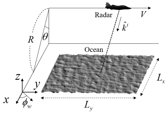
The geometric relation between the radar and the ocean surface is shown in Fig. 1. It is assumed that the radar moves along the y axis with a constant velocity, V. The range between the radar and the center point of the ocean scene is fixed as R over the integration time. The simulation dimensions of the ocean scene are L _x along the x axis and L _y along the y axis. k̂ ⁱ is the unit propagation vector of a microwave with an incident angle of θ on the ocean surface. φ _w is the wind direction. The range and azimuthal directions coincide with the x and y axes, respectively.

To generate the SAR image of the ocean scene, the time-varying ocean surface, Z(x, y, t) is generated as

where Ψ _mn = k _m x + k _n y − w _mn t + φ _mn , k _m = 2πm/L _x , and k _n = 2πn/L _y . ϕ is the fluid vector potential. A _mn is proportional to the square root of the ocean spectrum. Here, Fung and Lee’s spectrum is used [9]. φ _mn is a uniform random number over 0 to 2π, and wmn=g(km2+kn2) , where g is the gravitational acceleration, 9.81 m/s².

The ocean surface is discretized with many relatively large facets [7]. The motions of the ocean facet, such as particle velocity and acceleration, are computed as

The radial components of the particle velocity and acceleration are important on the SAR image and are given by u _r = k̂ ⁱ · u⃗ _p and a _r = k̂ ⁱ · a⃗ _p , respectively.

The normalized radar cross-sections (NRCS) by the ocean facets are calculated based on the combined model of the Kirchhoff approximation and the small perturbation method [10] as

Here,

where q⃗ = −2k ₀ k̂ ⁱ = [q _x , q _y , q _z ]. Prob (·, ·) is the slope probability density function [9]. Polarization-dependent parameter, α _mn (m, n = h or v) is related to the Fresnel reflection coefficients [10]. Here, h and v denote horizontal and vertical polarizations of the incident microwave, respectively. If the ocean scene changes in time, the local incident angle also varies, and yields the time-dependent NRCS. This time dependence can be easily considered when the ocean surface, (1) is computed at the time sampling points in the TD formulation. The ensemble-averaged SAR intensities can be obtained using analytical formulations, as shown in Section III.

The SAR image is not a one-to-one map of the imaged scene of the ocean surface [5]. The particles on the ocean surface cause the non-uniform displacement along the azimuth direction of the image plane because of the orbital motion [11], which generates wavelike patterns in the SAR image known as the VB mechanism. The TD model for SAR image is expressed as [6],

where T and k ₀ are the integration time and the microwave wavenumber, respectively. h is a pulse shape function in the range direction that can be approximated as h(x − x′) = δ(x − x′) [6]. The other parameters in (5) such as a, b, α, and γ are defined as

where τ _s is the coherence time of the ocean scene that is dependent on the phase speed or orbital velocity of the ocean wave [11]. (5) is calculated at every pulse repetition interval (PRI), which can allow accurately consider the variation of the ocean surface. However, the computation is time-consuming.

As the VB model is valid for the short integration time, the following approximations can be assumed: the time-dependent σ ₀ (x′, y′, t) is replaced by the mean σ̄ ₀ (x′, y′) over the integration time. u _r and a _r are expanded at about t = y/V in a Taylor series as a _r (x′, y′, t) ≈ a _r (x′, y′) and u _r (x′, y′, t) ≈ u _r (x′, y′) + a _r (x′, y′)(t − y / V), respectively [3]. With these approximations, (5) can be analytically simplified as [6]

where ρ _a ′ is the degraded azimuthal resolution as

To apply the VB model to a large integration time, time is divided into relatively short times, in which the velocity bunching model is valid. Thus, the final SAR intensity can be approximated as

where T _i is the divided time. N _TD and N _VB are the number of sampling times for the TD model and for the VB model, respectively.

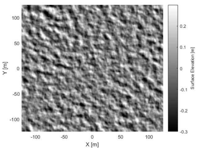
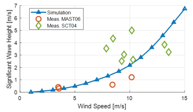
The generated ocean elevations are shown in Fig. 2 for a wind speed of 5 m/s. The scene dimension is L _x = 250 m by L _y = 250 m and discretized every 1 m sampling interval. The wind direction is assumed as φ _w = 45°. To validate the simulated ocean elevations, the significant wave heights (SWH) are compared with the measurement [12] for various wind speed. Fig. 3 shows the comparison between the simulation and the measurement. The measurement is carried out in the southern ocean near Port Lincoln, South Australia in August 2004 (SCT04) and in the ocean near Darwin in the Northern Territory in May 2006 (MAST06) [12]. The SWH of the simulated ocean surface agrees well with measurement results. The discrepancy for a few measurement points is due to the Fung and Lee spectrum, which assumes that the ocean is fully developed, that is there is no swell and the wind has sufficient fetch and duration for the ocean surface to reach equilibrium [12].

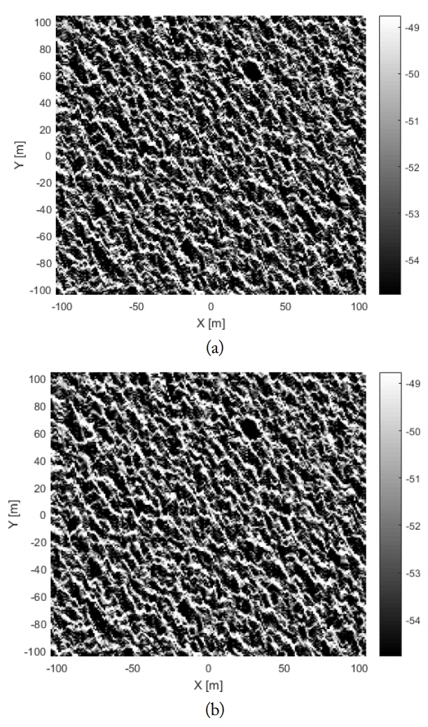
The simulation parameters are listed in Table 1. The SAR image intensities of the ocean surface by a 5 m/s wind speed are evaluated by the TD and VB models with R/V = 10 seconds and T = 0.2 seconds, and HH-polarization (see Fig. 4). The SAR images generated by two formulations have similar wavelike patterns and image intensity levels. Therefore, the VB model is accurate for such a short integration time as aforementioned T = 0.2 seconds.

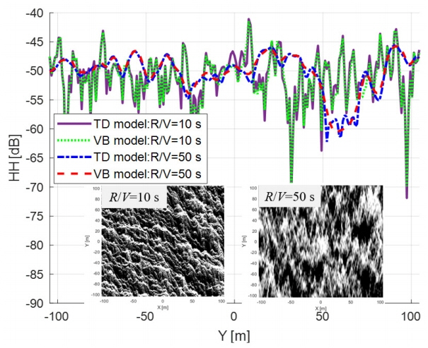
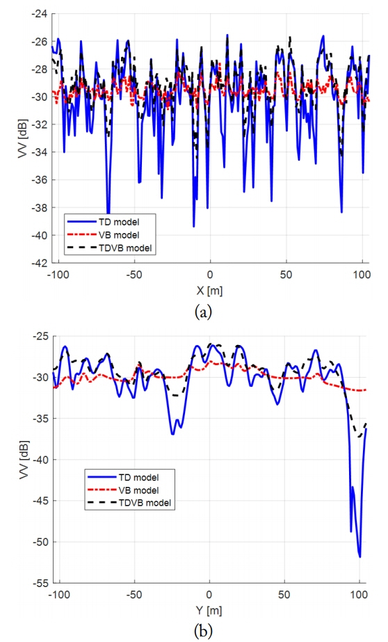
The SAR images for the 10 m/s wind speed are simulated for the following cases: R/V = 10 seconds and R/V = 50 seconds, T = 0.2 seconds and HH-polarization. The SAR images along the y axis at x = 0 are compared in Fig. 5 with the VB SAR images with two R/V ratios. The excellent agreement of the SAR image intensities by the TD and VB models is presented in Figs. 4 and 5. For a high R/V ratio, a strongly smeared SAR image intensity is observed along the azimuthal direction (Fig. 5). The motion by the ocean particles results in the image shift and compression along the azimuthal direction (see (7) and (8)). The smearing effect and the image shift of the SAR image becomes dominant as the R/V ratio increases as expected in (8). To simulate the SAR image for a large integration time, we assume R/V = 50 seconds, T = 6 seconds, VV pol and 5 m/s wind speed. The SAR images by the TD, VB, and time-divided VB (TDVB) models are compared in Fig. 6.

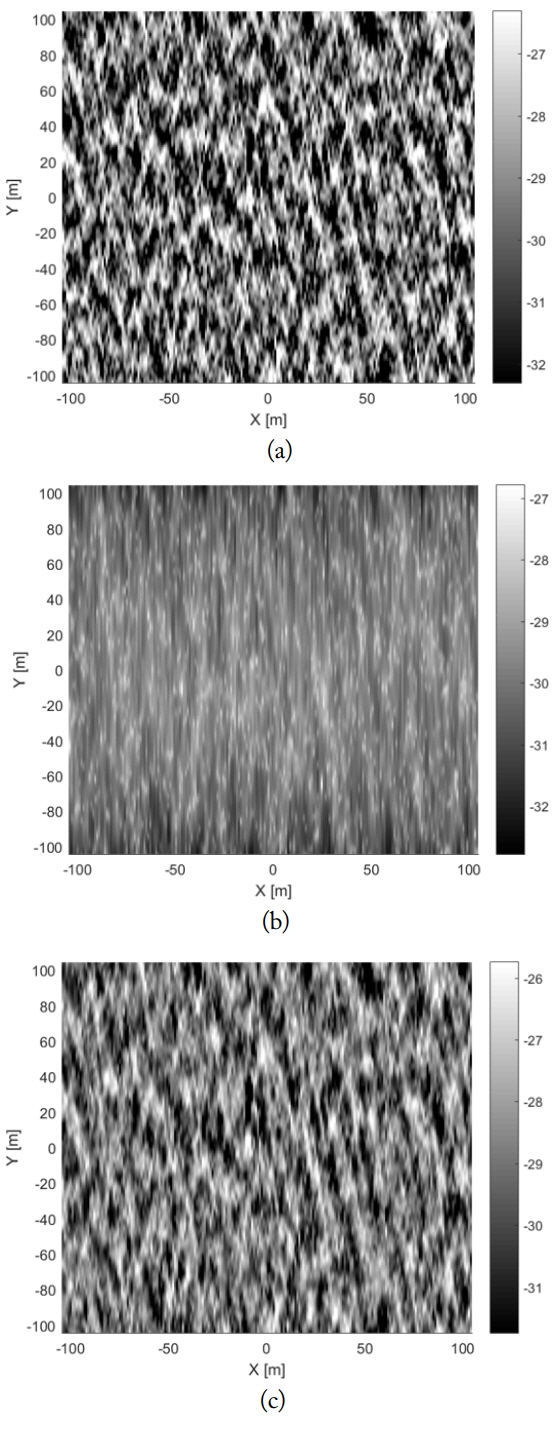
The results by the TD and TDVB models are in good agreement. Conversely, the VB model provides a more smeared SAR image. The comparison of the SAR intensities is shown in Fig. 7 along the x axis at y = 0 and along the y axis at x = 0.

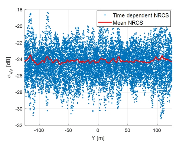
The SAR intensity by the VB model has fewer fluctuations because the VB equation assumes the time-independent particle velocity and acceleration as well as the mean NRCS during the integration time. In general, the time variation of the NRCS is large over the large integration time because of the ocean motion as seen in Fig. 8. These types of physical approximations reduces the image fluctuation of the VB model in comparison with the TD model, as shown in Fig. 7. The TD model is computed at every PRI, which is 1 ms in this study. Thus, for a 6-second integration time, 6,000 ocean surfaces (N _TD = 6,000) are generated for the TD model. Then the images are computed and merged into a final SAR image. But the TDVB model can generate an accurate SAR image with a much larger integration time than the PRI.

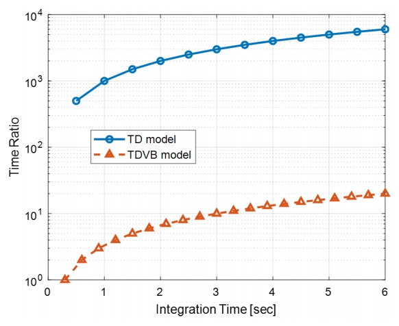
The determination of the proper integration times for the VB model is crucial because it affects to the model’s accuracy, which physically depends on how fast the ocean scene varies, i.e., scene coherence time, τ _s . Based on many simulations, 0.3 seconds is chosen as the optimal integration time for the VB model when τ _s = 0.1 seconds. Hence, TDVB model requires only 20 ocean scenes (N _VB = 20) for the 6 seconds integration time. Fig. 9 shows the simulation times consumed for the SAR image generation by the TD and TDVB models as a function of integration time when τ _s = 0.1 seconds. The TDVB model is around 300 times faster than the TD model over the entire integration time.

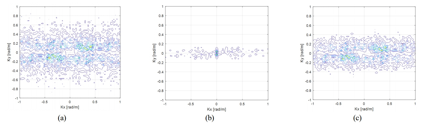
Fig. 10 shows the 2D spectra of the simulated 2D SAR images. As the fluctuation of the VB model is relatively small as observed in Fig. 7, the spectrum of the VB model is located at the low frequency range of Kx = 0 and Ky = 0. However, the other SAR image spectra of the TD and TDVB models spreads at a wider frequency range because of the consideration of the dynamic motion of the ocean surface over large time intervals.

The determination of divided sub-integration times for the TDVB formulation to generate accurate SAR images strongly depends on the scene coherence time, τ _s . Based on our heuristic simulations, the optimal integration times are evaluated with respect to various τ _s , which are summarized in Table 2. Note that higher integration time intervals are required as τ _s increases. As the ocean scene changes slowly when τ _s increases, which results in the small variation of the NRCS during an integration time, the valid integration time for the VB formulation increases.

In this study, an efficient formulation for the SAR image intensity is proposed based on the conventional VB model for a large integration time. The VB model is valid for a relatively short integration time but accurately considers the motion of the ocean in accurate fashion. Therefore, the VB model is repeatedly applied for a relatively large interval. Then, the generated images are merged into a final SAR image. This scheme is similar to the original TD model, applied at every radar PRI. However, the proposed scheme, the so-called TDVB model, generates ocean SAR images at a much larger interval than PRI, the numerical efficiency of which is much improved. Based on many simulations on realistic SAR scenarios, the optimal integration times of the VB model are proposed for various scene coherence times. The proposed image formulation is verified in several SAR scenarios such as ocean surfaces driven by two wind speeds of 5 m/s and 10 m/s, and different SAR parameters. The VB model is accurate for a short integration time. However, by increasing the integration time, the VB model cannot generate the correct SAR images. Conversely, the proposed formulation can generate accurate SAR images independently at the integration time. The SAR spectrum of the TDVB model is comparable with the TD SAR image.

Overcoming the fundamental limitation of the original VB model, which is valid only for short integration times, the TDVB model is applicable to a variety of SAR imaging applications with high numerical efficiency.