J. Electromagn. Eng. Sci Search

CLOSE


J. Electromagn. Eng. Sci > Volume 22(5); 2022 > Article
Jang and Cho: Spatial Delay Line Canceler-Based Sidelobe Blanking for Low Radar-Cross-Section Target

Abstract

This study proposes a sidelobe blanking (SLB) system with a spatial delay line canceler (DLC) and non-coherent integrator in a uniform linear array. After the equations for the target and noise power in the SLB system were established, SLB-ratio functions for the proposed and conventional SLB channels were developed. Using these ratio functions, the optimal SLB thresholds for the general detectable target and low radar-cross-section (RCS) target were estimated. The results of the SLB thresholds were confirmed by the Monte Carlo simulation, which indicated that the proposed SLB channel provides reliable performance without false SLB decisions in the sidelobe region. Using the estimated optimal threshold, the proposed SLB channel provides reliable performance, particularly for low-RCS targets. In contrast, the conventional SLB channel produces numerous false SLB decisions in the sidelobe region. The proposed synthesis is a simple but powerful method for obtaining the reliable SLB ratio. The SLB channel in various array antenna systems can be developed based on this method.

I. Introduction

A radar detects a target in a desired direction by transmitting and receiving radio waves. This means that the antenna of the radar maximizes the directivity of the detection direction and suppresses the other directions using a tapering window. Hereafter, in this study, the antenna beamwidth centered on the detection direction is referred to as the mainlobe, whereas the suppressed region excluding the mainlobe is referred to as the sidelobes.
In addition to signals from the mainlobe, the antenna simultaneously receives suppressed signals from the sidelobe. Despite the directivity of the antenna, the target signal in the mainlobe may still be indistinguishable from the clutter signals suppressed in the sidelobe because of the inherently low radar cross-section (RCS) of the target. If these unwanted signals from the sidelobe are not deleted or blanked during post-processing, it may result in false targets or system degradation of the radar.
To blank the sidelobe signals, radars use a sidelobe blanker (SLB). For this purpose, radars make an auxiliary channel for the SLB channel in addition to the detection channel and compares the output magnitudes of the detection and the SLB channels. Hereafter, the detection channel is referred to as the main beam channel, which forms the mainlobe on the detection direction. The SLB system first sorts out the mixed sidelobe signal in the main beam channel and then blanks it [1, 2].
Although an SLB channel generally requires a dedicated antenna, a phased array antenna can re-synthesize the outputs of the array for the SLB channel without an additional antenna. In addition, it can simultaneously apply adaptive beamforming to the main beam and SLB channels for nulling interference.
In this study, we focused on synthesizing a robust SLB channel for low-RCS targets. The synthesized SLB channel should be simply implementable to be expansible for adaptive beamforming. We designed this channel using a discrete Fourier analysis of spatial frequency and a finite impulse response (FIR) filter system in discrete time.
Digital signal processing (DSP), which samples time signals in a fixed sampling period, has a discrete sequence. Thus, assuming an equally spaced array, such as a uniform linear array (ULA) and far-field radiation, we can analyze array processing using the DSP technique. Some studies have already offered a fundamental understanding of digital array processing with FIR filtering [3, 4]. In addition, many applied studies have also been published.
Within the domain of array processing, adaptive beamforming has been investigated in diverse research fields. For radar, the objective of adaptive beamforming is to preserve detection performance under conditions of strong jamming or interference. Therefore, an adaptive SLB channel should be adopted for preserving the target through adaptive beamforming in the main beam channel; otherwise, the target will inevitably be blanked by strong interference in non-adaptive SLB channel. This requirement has resulted in various adaptive SLB studies [69]. While one study generalized adaptive detection using a generalized likelihood ratio test (GLRT) for SLB [6], another described a 2D adaptive sidelobe blanker (ASB) using the generalized adaptive coherence/cosine estimator (ACE) [7]. Yet another study modified the 2D adaptive matched filter (AMF) and ACE detector introduced in the aforementioned study using subarrays [8]. Suitable thresholds were presented for the detection margin, and results were achieved based on the designed subarrays.
Although research on adaptive methods for SLB is abundant, studies on channel synthesis for actual implementation are rare. We proposed an adaptive SLB channel synthesis in a ULA system using spatial delay line cancelers (DLC) and non-coherent integrators [1013]. The synthesis is simple but powerful in terms of the ratio difference between the channels, also called the detection margin [8]. In this study, we formulated SLB thresholds appropriate for low-RCS targets with equations for the signal-to-noise ratio (SNR) in the SLB system. We verified the performance using Monte Carlo simulations for all angles of the various target scenarios.
Practically, in a phased-array antenna system, the physical phenomenon of array mutual coupling and inaccurate calibration produces a substandard final array pattern, such as the main beam shape and the sidelobe level (SLL). Despite sound theoretical synthesis, inferior SLL performance causes degradation of SLB. Therefore, we focused on robust synthesis with a sufficient ratio difference for all angles to overcome this practical problem.
Section II summarizes the SLB channel synthesis proposed in an earlier study [12], while Section III presents the equations of the target signal, noise signal, and ratio for the SLB decision. Following this, Section IV presents the SLB thresholds suitable for the target signals and the results of the Monte Carlo simulation. Finally, Section V concludes the study.

II. Adaptive SLB Channel Synthesis

1. Conventional SLB System

To generate a good SLB performance, the angular pattern of the SLB channel should be distinguishable separately from that of the main beam channel in terms of the angular region, as displayed in Fig. 1. If this difference is insufficient, clutters with large RCS originating from the sidelobe region cannot be blanked, which may result in numerous false targets in theca main beam channel. Therefore, proper SLB channel design is critical for the optimization of the main beam of the radar system.
Fig. 1 displays the typical angular gain patterns of the main beam and SLB channels. The gain pattern of the SLB channel is smaller than that of the main beam channel in the mainlobe, which is the detection region, whereas the pattern is larger than that of the main beam channel in the sidelobe region. Fig. 2 presents a block diagram of a radar SLB system, in which the SLB decision compares the ratio of main2 (the output power of the main beam channel) to slb2 (the output power of the SLB channel) with a threshold of THSLB [1, 2]. If main2, represented by the solid line in Fig. 1, is smaller than THSLB compared to slb2, which is represented by the dotted line in Fig. 1, the main2 is assumed to originate from the sidelobe region and is eventually blanked. Since the actual signal of the mainlobe in the main beam channel exhibits maximum antenna gain, it is always greater than the output of the SLB channel.
(1)
SLBblankmain2ifmain2slb2<THSLB,processmain2otherwise.
where,
  • main: output of the main-beam channel,

  • slb: output of the SLB channel,

  • THSLB: threshold of the SLB decision.

2. Adaptive SLB System with Spatial DLC and Non-coherent Integrator

As mentioned earlier, to obtain a clear SLB decision, the main beam channel should be sufficiently greater than the SLB channel in the mainlobe. In this study, we set the decision criterion as THSLB and designed a distinguishable angular pattern of the SLB channel in the overall angular domain. Fig. 3 depicts an adaptive SLB channel synthesized in a ULA system, along with the spatial DLC and non-coherent integrators [12].
A DLC in the Doppler domain is a simple and powerful tool for indicating a moving target. Thus, it was applied to the spatial domain. A spatial DLC forms a null at the boresight ϕlook of the angular pattern in the same manner as the DLC does on the zero Doppler. The proposed SLB synthesis is summarized as follows: first, the null makes a significant gap between the two channels within the mainlobe. Second, in the sidelobe region, the non-coherent integrator makes the angular pattern of the SLB channel uniformly higher than that of the main beam channel. Finally, adaptive beamforming ensures robust SLB performance in environments with interference.
In this section, we briefly describe the spatial DLC response, which is explained in further detail in Fig. 4. The DLC operation is called the first difference in discrete time [14]. Each sample in the output signal is equal to the difference between the two adjacent samples in the input signal. Using this operation, we defined the spatial DLC system in the ULA with the impulse response hsDLC [n] and frequency response HsDLC (u), where n is the element number in N-element ULA, and u is the spatial frequency in period us.
(2)
hsDLC[n]=δ[n]-δ[n-1]DTFTHsDLC(u)=1-exp(-j2πu/us)=exp(-jπu/us)·(2j·sin(πu/us))
Owing to the zero value of sin(πu/us) at u = 0 in HsDLC (u) with ulook = 0, the angular pattern of the adaptive SLB channel is considerably different from that of the adaptive main channel. Therefore, main2/slb2 is clearly distinguishable between the mainlobe and the sidelobes, thus improving SLB decisions.

III. SLB-Ratio Function for SLB Decision

In this section, we present the SNR of each input/output signal as well as the SLB ratio formulation in the proposed SLB system. To simplify the equations, we assumed the boresight φlook = 0° of the array and omitted adaptive beamforming.
As mentioned previously, we developed formulations of the N-element ULA using a discrete-time Fourier transform (DTFT) or DSP technique, with n = 0,1,…N-1 in the spatial/array domain and u along with period us in the spatial frequency domain. However, in this study, we did not consider the time variables in each element or the array system. Note that variable n represents the sample or element number in the spatial/array domain and is not related to time. A former study has explained the DSP technique in terms of the sample domain [17].

1. Impulse Response and Frequency Response of the SLB System

In the N-element ULA, the signal field arriving from φ is measured at locations d · n of N elements with spatially equal distance d, expressed as:
(3)
r(n,φ)=a(n,φ)·p(n,φ)n=0,1,N-1=α·p(n,φ)
where a(·) and p(·) represent the amplitude and phase distributions of the elements, respectively, while φ is the arrival angle perpendicular to the ULA. For isotropic and far-field radiation, the distribution of a(·) is uniform over all n and becomes a constant α. The phase difference between the adjacent elements is consecutively delayed, corresponding to the direction of φ. This denotes the response of the array, which can be expressed as follows:
(4)
p(n,φ)=exp(j2π·sinφ/λ·d·n)Or p(n,u)=exp(j2πu/usn)
where λ and d represent the wavelength of the signal and the equal distance between the elements, respectively.
N samples of the measured signal in the ULA have a fixed spatial sampling distance of d between samples, spatial frequency u = sinφ/λ by equal phase difference between samples, and a spatial sampling frequency of us = 1/d [5, 12].
(5)
r(n,u)=α·exp(j2πu/usn)n=0,1,N-1
The output of the array eventually constitutes a discrete sequence of r(n, φ) satisfying the DSP technique, and can produce a function of spatial frequency u through DTFT.
Spatial domain of the array (n=0,1,N-1)DTFTSpatial frequency domain (uperiodic with us)Inverse DTFT:
Inverse DTFT:
(6)
r[n]=-us/2us/2R(u)·ei2πuusndu
where
(7)
R(u)=nr[n]·e-i2πuusn
r[n] represents a discrete set of samples r(n, φ) measured in each element.
Fig. 4 displays a block diagram specifying the mathematical expressions for the input/output signal and the impulse responses of each stage in the proposed SLB system. For the target signal, x[n] denotes the output set of the array and input set of the SLB system, y[n] denotes the output set of the spatial DLC in the proposed SLB channel, while z(φ) denotes the output of the beamformer in the main beam channel for detection. The noise signals are denoted as nx[n], ny[n], and nz(φ) with respect to the target signal. Furthermore, the final output signals of each channel are denoted by main2 and slb2, in which the target and noise are still mixed.
We denote the impulse responses of the spatial domain and the spatial frequency responses in each channel using Eqs. (6) and (7). In this context, hB[n] and HB(u) indicate the beam-former in the main-beam channel, whereas hS[n] and HS(u) refer to the spatial DLC in the SLB channel. We define the normalization constants αBF and αsDLC, respectively, for the constraint “noise gain = 1.”
(8)
hB[n]=αBF·hBF[n],         αBF=1k=0N-1hBF[k]2hB[n]DTFTHB(u)=αBF·HBF(u)
(9)
hS[n]=αsDLC·hsDLC[n],αsDLC=1k=12hsDLC[k]2hS[n]DTFTHS(u)=αsDLC·HsDLC(u)
Since the SLB system satisfies the conditions for DTFT, which particularly has an equal spatial sampling distance of d for all n, it can also be considered for digital FIR filtering. hB[n] represents a filter matched to the array response vector for the boresight φlook = 0º as well as the conventional frequency-selective digital filter of finite length [5]. This indicates that we can design N coefficients of hB[n] for the directivity to reach a maximum frequency response at ulook = sin φlook/λ = 0. Similarly, we can observe the hS[n] of Eq. (2) as the frequency-selective FIR filter, with two coefficients for the frequency response with the null at ulook= 0. In addition, for causality, we designed the length of the FIR filter in such a way that the nth output uses only the samples of the ith elements, with in at an observation time, as in Eq. (2). Thus, the designed FIR filter is causal for n.
Eq. (10) shows the general form of the output g[m] in a causal discrete FIR system, which is analogous to the discrete convolution of f[m] with coefficients of h[m] in Eq. (11) [1416]:
(10)
g[m]=k=0M-1bkf[m-k]
(11)
h[m]={bmm=0,1,,M-1,0otherwise.
The impulse response h[m] has a finite length of M.
This general form can be used to obtain the output of the FIR filter in Fig. 4, according to the discrete input sequence of r(n, ui) in Eq. (5):
(12)
g[n]=k=0M-1hx[k]·r[n-k,ui]=α·exp(j2πuiusn)r(n,ui)k=0M-1hx[k]exp(-j2πuiusk)Hx(ui),
where g[n] represents the output of a FIR filter, hx[n] denotes any impulse response in Fig. 4, and ui is the spatial frequency of the input samples related to the arriving direction φ.
Since the input set r[n, ui] is a complex exponential, the nth output g[n] finally represents the multiplied form of the nth input sample r(n, ui) and Hx(u) at ui: Hx(u) represents the spatial frequency response of M-length hx[n] FIR filter. Specifically, Hx(ui) indicates the value of the frequency response designed for frequency-selectivity according to the input spatial frequency. Eq. (12) can be further understood with digital FIR filtering as follows: the length of the frequency-selective FIR filter, and the steady-state response of the FIR system:
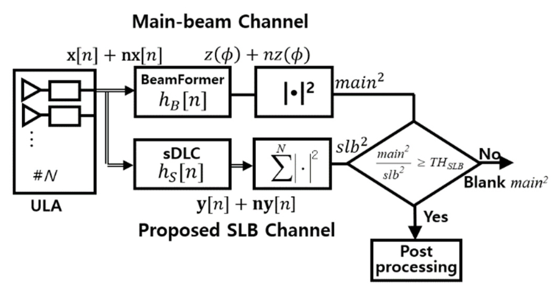
  1. We designed the M-length of hx[n] to extract the desired spatial frequency-selective response, for example, the directivity and the null. Thus, the number of valid output samples depends on the M. If M is greater than the number of input samples N, we cannot obtain the valid output with the designed frequency-selective response of MN, which is a necessary condition for Fig. 4. In the spatial DLC in the SLB channel, the output y[n] has valid output samples of N-1, n = 1,..., N-1, since hS[n] satisfies the causality of the first difference operation and is 2-length in Eq. (2). In the case of the beamformer in the main beam channel, for Nlength hB[n], the only N-1th output is valid:

    (13)
    z(ui)=g[N-1]=k=0N-1hB[k]x[(N-1)-k]=x(N-1,ui)·HB(ui)=αxexp(j2πui/us)·(N-1))·HB(ui)
    The output with one sample no longer has a variable of n in the spatial domain, and is related to the spatial frequency response at ui, as in Eq. (13).
  2. If the input of the FIR system is a complex exponential, as in Eqs. (5) and (12), the Hx(ui) in the output is referred to as the steady-state response of the system [14]. It represents the spatial frequency response at ui in steady state, such as a pass-band or a stop-band. In addition, the steady state indicates holding its frequency response for all observations [1416]. Consequently, the Hx(u) with the input-complex-exponential must persist for n of any output. In particular, the steady state response Hx(u) has no more statistical meaning, such as averaging over n. On the other hand, the first term in Eq. (12), representing the value of the current input sample, becomes only a factor for scaling the amplitude and shifting the initial phase independent of the system response. Therefore, it is regarded as an ignorable complex constant of the system response.

2. Target Signal

The target signal sampled at each element, x(n, ut), refers to the complex exponential form generated along with the target’s amplitude and spatial frequency [19]:
(14)
x(n,ut)=σtexp(j2πut/usn)n=0,1,N-1
where
  • σt: RCS or amplitude of the target,

  • ut = sin(φt)/λ : spatial frequency of the target,

  • φt: arriving angle of the target.

As in Eq. (3), the instant amplitude of x(n, ut) at an arbitrary time has the same deterministic value σt for all n. Thus, we obtain the target’s input power of x[n] in Fig. 4:
(15)
Px=E{x[n]2}=σt2E{|exp(j2πutusn)|2}=σt2
where E{·} denotes the expected value for all n in the spatial domain.
We summarize the target output signal in the proposed SLB channel. First, using Eqs. (9) and (12) , the output set of the spatial DLC y[n] consists of:
(16)
y[n]=k=1N-1hS[k]·x[n-k]n=1,2,,N-1=σt   exp(j2πutusn)·HS(ut)
According to the null at ulook= 0 in Eqs. (2) and (9), if the target of y[n] is on the boresight ut = ulook, the frequency response HS(ut) becomes zero, that is, y[n] = 0, if ut = ulook.
Next, the proposed SLB channel passes y[n] through the non-coherent integrator, which calculates the energy of y[n] through the total sum of the input power, as specified in Fig. 4. We obtain the target output signal for slb2 by employing Êy, the modified energy by αN.I to satisfy the noise normalization constraint in Eq. (18).
(17)
Ey=k=1N-1y[k]2=(N-1)·σt2HS(ut)2
(18)
E^y=αN.I·Ey         αN.I=1/(N-1)
Finally, we obtain the target output signal for main2 in Fig. 4. The output power in main2 can be mathematically expressed as the squared magnitude of the beamformer—the output signal z(u) of the main beam former is in accordance with z(φ). As mentioned in the steady-state response of the FIR system with complex exponential inputs, the expected value of the output z(u) for all n becomes unimportant. Therefore, we obtain the target output signal in main2 as power Pz:
(19)
PZ=z(ut)2=σt2·HB(ut)2

3. Noise Signal

Contrary to a target signal with a deterministic amplitude, the expected value for all n can be calculated using an autocorrelation function, since noise power is a random variable [1416]. Let σn2 and m be the average noise power in the output of each element and the lag amount of the autocorrelation function, respectively. Since nx[n] is uncorrelated between the elements, the autocorrelation function ρnx,nx(m) can be expressed as follows:
(20)
ρnx,nx[m]=σn2·δ[m]
The average power of nx[n], Pnx, is considered to be equal to the autocorrelation function’s quantity at m = 0:
(21)
Pnx=E{nx2[n]}=ρnx,nx[0]=σn2
For the output noise signal ny(n) of the spatial DLC, the autocorrelation function and its average power are denoted as follows [1416]:
(22)
ρny,ny[m]=ρny,ny[m]*hS[m]*hS*[-m]
where * is a discrete convolution and * represents a complex conjugate.
(23)
Pny=E{ny2[n]}=ρny,ny[0]=σn2k=12hS(k)2
For the final output noise in slb2 by the non-coherent integrator, we obtain the energy of the input noises, Eny = (N − 1)Pny, as in Eq. (17), and then normalize it using the noise constraint constant αN.I:
(24)
E^ny=αN.I(N-1)Pny         αN.I=1/(N-1)
Next, we consider[ the noise signal in main2. The output noise set nz(n) of the beamformer can be represented in the same manner as Eqs. (22) and (23).
(25)
ρnz,nz[m]=ρnx,nx[m]*hB[m]*hB*[-m]
(26)
Pnz=E{nz2[n]}=ρnz,nz[0]=σn2k=0N-1hB(k)2
Finally, we review the output noises Êny and Pnz of the two channels, along with the noise constraint constants.
(27)
E^ny=Pny=σn2k=12hS(k)2Pnz=σn2k=0N-1hB(k)2
where
k=12hS(k)2=αsDLC2k=12hsDLC(k)2=1k=0N-1hB(k)2=αBF2k=0N-1hBF(k)2=1
Though the output noises Êny and Pnz have individual gains in proportion to the input noise power σn2, all gains become “unit gain = 1” by αsDLC and αBF. Therefore, all output noises in Fig. 4 have the same value of σn2.
(28)
Pnx=Pnz=Pny=E^ny=σn2

4. Input/Output SNR and SLB-Ratio Function

This section presents the input and output SNRs of each channel as well as the SLB ratio between the two channels for the SLB decision using equations of the targets and noise signals. For the performance comparison, the output SNR of the conventional SLB channel, SNRslb_conv, is further defined as Eq. (32). We assume that the conventional SLB uses the one-element output of the array antenna or the non-coherent integrator of the elements with noise normalization [9], SNRslb_conv, which has the same SNR as the input. The input/output SNR can then be expressed as:
Input SNR of the SLB system, as shown in Fig. 4:
(29)
SNRin=Px/Pnx=σt2/σn2
Output SNR of the main beam channel:
(30)
SNRmain=Pz/Pnz=SNRin·HB(ut)2
Output SNR of the proposed SLB channel:
(31)
SNRslb=E^y/E^ny=SNRin·HS(ut)2
Output SNR of the conventional SLB channel:
(32)
SNRslb_conv=Px/Pnx=σt2/σn2=SNRin
Next, we derive the SLB ratio of main2 to slb2 for the SLB decision. The target and noise signals in the channel were mixed and were found to be uncorrelated, indicating that they are independent variables. Therefore, the average power of the channel can be obtained by adding the average power of the target and the noise.
The expected value of the SLB ratio E{Ratio} between the output powers of the two channels is summarized in Eq. (33) by noise normalization, depending on the output SNRs of the two channels.
(33)
E{Ratio}=E{main2slb2}=Pz+PnzE^y+E^ny=Pz/Pnz+1E^y/E^ny+1=SNRmain+1SNRslb+1
Substituting the equations of the output SNRs, we can obtain the SLB ratios depending on the SNRin, ut, and the spatial frequency responses of two channels, as follows:
(34)
E{Ration}=SNRin·HB(ut)2+1SNRin·HS(ut)2+1
Extending ut to the entire spatial frequency domain, we can compare the SLB ratio functions between R(·) of the proposed SLB and Rconv(·) of the conventional SLB.
(35)
R{u,SNRin}=SNRin·HB(u)2+1SNRin·αsin(πuus)2+1
where α is 2, as indicated by Eqs. (2) and (9).
(36)
Rconv{u,SNRin}=SNRin·HB(u)2+1SNRin+1
The different component of Eqs. (35) and (36) is the sin(πu/us) term of HS(u) in the denominator, which creates a null at u = ulook. Thus, for a target near ulook, the R(·) may be approximated to SNRmain, which is significantly greater than Rconv(·): if utulook, R(ulook) >> Rconv(ulook). However, for a target in the sidelobe region, it becomes gradually smaller because of sin(·). Compared to Rconv(·), R(·) provides a distinguishable ratio with respect to u and then ensures an excellent SLB performance, which ultimately decides whether the target originates from the sidelobe or otherwise.
The various target scenarios for the SLB ratios are listed in Table 1, while the SLB ratios of Eqs. (35) and (36) are illustrated in Fig. 5. We employed the Taylor window with an SLL of 30 dB for tapering in a 16-element ULA.
For Case 2 in Table 1, the target with a 13-dB SNRmain represents a commonly minimum-detectable target in the radar detector. The signal would be injected with 1.65-dB SNRin at the input of the beamformer to obtain SNRmain = 13 dB at ulook for this simulation. Compared to the minimum-detectable target with 13-dB SNRmain in Case 2, Case 3 represents a more easily detectable target with 3-dB higher power, while Case 1 represents a low-RCS target with 3-dB lower power.
We generated the target signal arriving from the individual u of all u and then calculated the SLB ratios in Fig. 5. For the ulook within the mainlobe, R(·) in (a) has a large value close to SNRmain, but the Rconv(·) in (b) has a relatively low value. Conversely, in the sidelobe region, R(·) gradually decreases to be lower than Rconv(·). Furthermore, for the identical target case, R(·) has a value that is 2–6 dB higher than that of Rconv(·) at ulook, and a lower value in the sidelobe. We can observe that R(·) provides considerably distinct ratios for various target scenarios according to SNRin.

IV. Optimal SLB Threshold and Simulation Results

In this section, we estimate the SLB thresholds suitable for the desired targets using the derived SLB-ratio function. The results are demonstrated through 10,000 Monte Carlo simulations.
For practical situations, a cos-shaped element pattern was used to simulate a target signal [20].
(37)
fe(ϕ)2=cos3/2φ

1. SLB Thresholds Appropriate for the Targets

The radar system generally regards a 3-dB beam width as the detection region, while the blanking region of an SLB indicates the regions that exclude the detection region. We determined the SLB threshold of the boundary separating the detection and blanking regions as the value of the SLB-ratio function at a 3-dB beam width of ±u3dB using Fig. 5.
Table 2 indicates the SLB thresholds—the SLB-ratio function’s value with respect to a wanted SNRin and ±u3dB. It is evident that Th 2 is applicable for the typical minimum-detectable target with 13-dB SNRmain, while Th 1 is appropriate for a low-RCS target with 3-dB lower power.
THSLB by R(·) of 10.23 and 7.5 dB refer to the proposed SLB channel, 6.5 and 5.4 dB by Rconv(·) refer to the conventional SLB channel in the simulations. The proper SLB thresholds by R(·) for the detection region are much higher than those by Rconv(·), thus performing robust SLB decisions in noisy environments or with the low-RCS targets. This is because the proposed SLB channel increases R(·) significantly within the detection region as mentioned previously. In contrast, 6.5-dB Th 2 by Rconv(·) has an insufficient difference relative to the noise even for the minimum-detectable target of 13-dB. Furthermore, Th 1 for a low-RCS target is severely lowered to 5.4 dB, we can predict that the lower threshold will lead to the performance degradation. The superiority of the SLB thresholds by the proposed SLB channel was verified in more detail in the simulation results.

2. Simulation Results

The Monte Carlo simulation generated the test signal with the noise at every u point of the target scenarios in Table 1, estimated the SLB ratio, and processed the SLB decision with reference to the SLB thresholds in Table 2. The same procedures were repeated 10,000 times at each u.
With reference to the figures depicted in this section, the legend “sDLC + NCI” pertains to the proposed SLB channel and “Conventional” pertains to the conventional SLB channel.
In (a) of Figs. 611, the y-axis of “Target Existence Decision#” denotes the number of decisions about the target-in-mainlobe at each u. Specifically, the SLB determines that the angle of the test signal is the mainlobe and does not blank it—it is interpreted as either the detectability of the target-in-mainlobe or the blanking ability of the target-in-sidelobe. This represents SLB performance at a specific u.
In (b) of Figs. 611, the y-axis of the “Probability mass function” represents the proportional quantity of “Target Existence Decision#” at each u to the total decisions taken in all u. It represents the probability density of “Target Existence Decision#” in the u domain, also known as the discrete density function [21]. This indicates the reliability of the SLB performance in a particular u compared to all other u domains. Notably, the probability mass function ftgtML(ûl) has a sum value of 1 for all u:
(38)
uι^=-0.50.5ftgtML(uι^)=1
where uι^Equation is u normalized with us, uι^=u/us.
We analyzed the performance results of the SLB synthesis and thresholds with the following indicators:
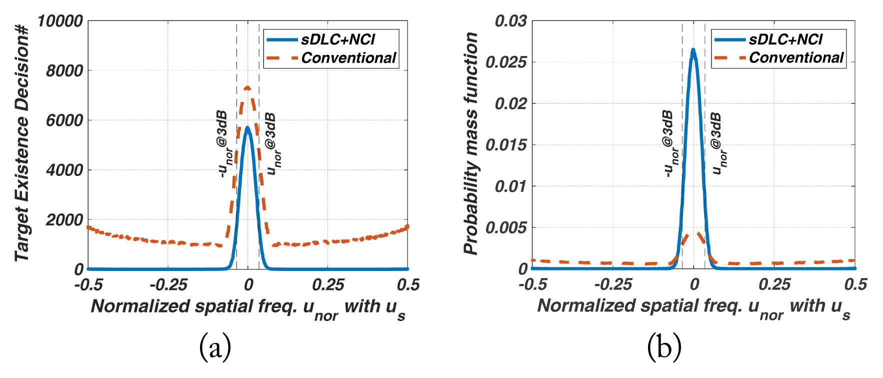
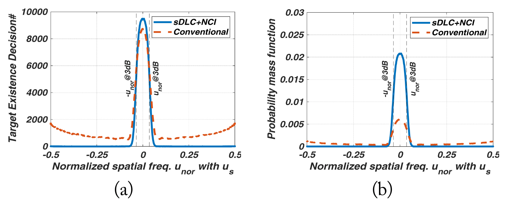
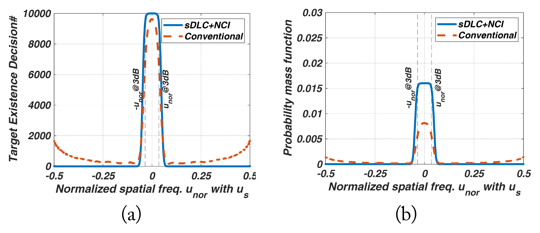
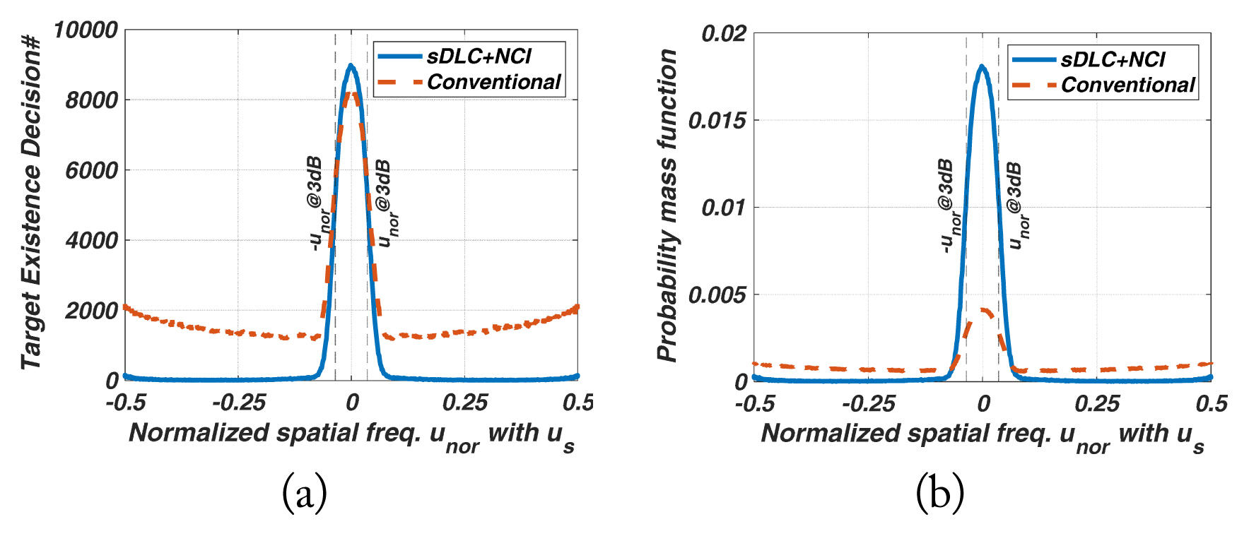
  1. The amount of “Target Existence Decision#” within ±u3dB represents the detectability of the target-in-mainlobe in the detection region, meaning the frequency of a target-in-mainlobe decision occurring in the mainlobe. If this value is low, many of the target-in-mainlobes are blanked by SLB, thus reducing the detection probability of a radar.

  2. The distribution of the probability mass function identifies the region where the decision probability of the mainlobe target occurs intensively.

  3. The partial sum of the probability mass function within ±u3dB involved a reliability in the detection region relative to the entire u domain. This is an important indicator of a low-RCS target because an improper SLB threshold or an insufficient SLB ratio can frequently blank the target with low SNRmain in the detection region. Thus, we have displayed the quantities in tabular form. Additionally, an unfavorable SLB ratio and SLB threshold of a low-RCS target are inherently difficult when it comes to satisfying overall performance. Hence, a reasonable threshold may be acceptable. Although there is a disadvantage of low detectability of “Target Existence Decision#” in the detection region, it is sufficient to satisfy fewer blanking errors and high reliability in the detection region. Nevertheless, in the proposed method, an appropriate threshold exhibits superior detectability with high reliability in the detection region.

  4. The remaining partial sum within the ±u3dB involved a blanking error in the blanking-region:

(39)
1-Σi±u3dBftgtML(ui)
Despite the blanking region, the SLB incorrectly makes a decision as the target-in-mainlobe and does not blank it. This further relates to the blanking ability of the target-in-sidelobe.

2.1 Results of the threshold appropriate for a minimum-detectable target

Initially, we set THSLB as Th 2 applicable for the typical minimum-detectable target in Table 2, the input target scenarios in Table 1 were simulated. The results are presented in Figs. 68 and Table 3.
For Cases 2 and 3 in Figs. 7(a) and 8(a), since the input targets have enough SNRmain of 13-dB or more for Th 2, “sDLC + NCI” and “Conventional” both exhibit good detectability of the target-in-mainlobe in the detection region. However, due to the false SLB decisions in the sidelobe region in the (a) of Figs 7 and 8, “Conventional” shows poor reliabilities across u compared to “sDLC + NCI”. In contrast, “sDLC + NCI” has the intensive shape of the probability mass function only within the detection region in (b)s, ensuring excellent reliability across u.
For Case 1 of a low-RCS input target in Fig. 6, its signal of a 10-dB SNRmain at ulook is significantly lower than that of Cases 2 and 3 as well as the target’s SNR subject to Th 2. Thus the estimated SLB ratio is also reduced relative to Th 2—meaning that we have an insufficient difference between the estimated SLB ratio in Case 1 and Th 2. Therefore, as observed in Fig. 6(a), the “Target Existence Decision#” occurred slightly in both “sDLC + NCI” and “Conventional.” More severely, “Conventional” increases the overall blanking error in the blanking region. However, “sDLC + NCI” still guarantees a good reliability across u in Fig. 6(b).
Specifically, in Table 3, “sDLC + NCI” of Case 3 has high reliability of 0.9 in the detection region despite the low detectability, owing to the lower SNRin—meaning that almost all decisions of the target-in-mainlobe occur correctly near ulook. Cases 2–3 of “sDLC + NCI” guarantee the reliability of 0.75 and 0.86 near the detection region, and moreover, Case 3 has perfect decisions of 10,000 near ulook. On the other hand, the reliability of “Conventional” in the detection region decreases from 0.35 and 0.25 for Cases 2–3 to 0.19 for Case 1, specifically indicating the deterioration of the overall performance with the lower SNRin.
Th 2 of “sDLC + NCI” has much better overall performance than Th 2 of “Conventional,” and is reasonable even for a low-RCS input target due to the high reliability in the detection region. The following section indicates that having an appropriate SLB threshold for a low-RCS target can improve the results of the “sDLC + NCI.”

2.2 Results of the threshold appropriate for low-RCS target with SNRdetectable = 10 dB

We reset THSLB as Th 1 ppropriate for a low-RCS target in Table 2, and equally simulated the input target scenarios. The results are presented in Figs. 911 and Table 4. We compared the results of different SLB thresholds Th 1–2 for the identical input targets. The value of Th 1 decreases with SNRin of a low-RCS target compared to the value of Th 2.
In the results of “Conventional,” comparing (a) of Figs. 68 and (a) of Figs. 911, numerous errors in the SLB decisions occur outside the detection region. Since a severe low value of 5.4 dB for Th 1 frequently considers the noise to false target. Besides, across all u, the “Target Existence Decision#” increases slightly owing to the lower threshold. Thus, using Th 1 instead of Th 2 improves detectability slightly better in the detection region, but significantly reduces the blanking ability in the blanking region. We also observe that the values of the probability mass function at ulook decrease further in (b) of Figs. 911, and eventually the reliability of the detection region of Case 1 deteriorates from 0.19 to 0.17 in Tables 34.
In the results of “sDLC + NCI”, Th 1 is significantly reduced by approximately 3 dB—from 10.23 to 7.50 dB. Therefore, comparing (a) of Figs. 68 and (a) of Figs. 911, the “Target Existence Decision#” increases remarkably across all u. Specifically, for Case 1 in Figs. 6 and 9, it increases by more than 30%: by 3,628 at ±u3dB and by 3,259 at ulook. Despite the 3 dB lowered threshold of Th 1, blanking error is rare in the blanking region unlike in the results of “Conventional”, thereby guaranteeing the superior reliability compared to Th 2. Furthermore, Cases 2–3 for Th 1 have perfect decisions of 10,000 within the detection region, and the distribution shapes become maximally clipped in the detection region by perfect decisions in Figs. 10 and 11. Note that the partial sums of “sDLC + NCI” decrease from the values for Th 2 in Table 3 to the values for Th 1 in Table 4. Since perfect decisions of the target-in-mainlobe are taken beyond the detection region, not within the detection region. In other words, reliability of Th 1 is only numerically low, and the performance is better than that of Th 2.

V. Conclusion

This study proposes the synthesis method for a robust SLB channel for low-RCS targets. This method is simply implementable to be expansible for adaptive beamforming. This method generates a distinguishable angular pattern with respect to the mainlobe and the sidelobe compared to the pattern of the main beam channel. The corresponding SLB ratio has remarkably changeable values with respect to the u domain, since it is increased at ulook by sDLC and decreased in the sidelobe region by the non-coherent integrator.
We also formulated an SLB-ratio function of u, SNRin, and the spatial frequency response and then estimated a suitable SLB threshold for the low-RCS target. The proposed SLB provides much better overall performance than the conventional SLB for various targets scenarios, especially reliability across u. Since the difference between the SLB ratio and the SLB threshold is ensured sufficiently by sDLC.
The proposed SLB also provides appropriate threshold for a low-RCS input target, guaranteeing both superior reliability without blanking error and the high detectability of the target-in-mainlobe in the detection region. The suitable threshold for a low-RCS target improved the SLB performance by more than 30% compared to the threshold for the typical minimum-detectable target. Furthermore, it improved reliable detectability in the detection region while guaranteeing blanking ability in the blanking region with a negligible error of under 0.15.
In contrast, even for the minimum-detectable target, the conventional channel exhibited a huge error of more than 0.75 in the blanking region. The blanking error of the threshold for a low-RCS target became more severe, increasing up to 0.83. Therefore, the conventional SLB cannot provide reliable performance for a low-RCS target. As a result, we focused on the novel synthesis of an SLB channel for a low-RCS target.
We applied a cos-shaped element pattern to the actual array modeling. However, there are more considerable realistic errors, such as errors by the Swerling target model, physical array error of mutual coupling, and inaccurate calibration. These challenges can be addressed by sufficient SLB ratio differences owing to spatial DLC, which can be easily implemented. Therefore, we can consider developing it in complex antenna systems, such as sub-arrays or planar arrays, based on the synthesis proposed in this study.

Fig. 1
Angular gain patterns of the main beam and SLB channels.
jees-2022-5-r-126f1.jpg
Fig. 2
SLB system of the radar.
jees-2022-5-r-126f2.jpg
Fig. 3
Comparison of the angular patterns between the adaptive main and the proposed adaptive SLB channels using the spatial DLC and non-coherent integrators: ULA with 16 elements, d = λ/2, and Taylor window (30 dB SLL). Adapted from [12].
jees-2022-5-r-126f3.jpg
Fig. 4
Block diagram of the proposed SLB system in the ULA.
jees-2022-5-r-126f4.jpg
Fig. 5
Graph of R(u, SNRin) and Rconv(u, SNRin) for the targets in Table 1: (a) proposed SLB channel and (b) conventional SLB channel.
jees-2022-5-r-126f5.jpg
Fig. 6
Results for Case 1 (input target with SNRmain = 10 dB at ulook): Th 2 for the target with SNRdetectable = 13 dB. (a) number of decisions as the target in the mainlobe and (b) probability mass function of (a).
jees-2022-5-r-126f6.jpg
Fig. 7
Results for Case 2 (input target with SNRmain = 13 dB at ulook): Th 2 for the target with SNRdetectable = 13 dB. (a) number of decisions as the target in the mainlobe and (b) probability mass function of (a).
jees-2022-5-r-126f7.jpg
Fig. 8
Results for Case 3 (input target with SNRmain = 16 dB at ulook): Th 2 for the target with SNRdetectable = 13 dB. (a) number of decisions as the target in the mainlobe and (b) probability mass function of (a).
jees-2022-5-r-126f8.jpg
Fig. 9
Results for Case 1 (input target with SNRmain = 10 dB at ulook): Th 1 for the target with SNRdetectable = 10 dB. (a) number of decisions as the target in the mainlobe and (b) probability mass function of (a).
jees-2022-5-r-126f9.jpg
Fig. 10
Results for Case 2 (input target with SNRmain = 13 dB at ulook): Th 1 for the target with SNRdetectable = 10 dB. (a) number of decisions as the target in the mainlobe and (b) probability mass function of (a).
jees-2022-5-r-126f10.jpg
Fig. 11
Results for Case 3 (input target with SNRmain = 16 dB at ulook): Th 1 for the target with SNRdetectable = 10 dB. (a) number of decisions as the target in the mainlobe and (b) probability mass function of (a).
jees-2022-5-r-126f11.jpg
Table 1
Target scenarios for the simulation (Element # 16, GSNR = 11.35 dB with Taylor 30 dB SLL)
SNRmain (dB) SNRin (dB)
Case 1 10 −1.35
Case 2a 13 1.65
Case 3 16 4.65

GSNR = SNR gain of the beamformer in the main beam.

SNRin = SNRmainGSNR

a A typical minimum-detectable target in the radar.

Table 2
SLB thresholds for ±u3dB (detection region) corresponding to a low-RCS target and a detectable target
SNRmain (dB) THSLB (dB)

R(u3dB, SNRin) Rconv(u3dB, SNRin)
Th 1 10 7.50 5.40
Th 2 13 10.23 6.50
Table 3
Partial sum of ftgtML(ui) within ±u3dB (Th 2)
Input target SNRmain at ulook (dB) i±u3dBftgtML(ui)

sDLC+NCI Conventional
Case 1 10 0.90 0.19
Case 2 13 0.86 0.25
Case 3 16 0.75 0.35

Th 2 (dB) = 10.23 (sDLC + NCI), 6.50 (Conventional).

Table 4
Partial sum of ftgtML(ui) within ±u3dB (Th 1)
Input target SNRmain at ulook (dB) i±u3dBftgtML(ui)

sDLC+NCI Conventional
Case 1 10 0.75 0.17
Case 2 13 0.70 0.23
Case 3 16 0.62 0.31

Th 1 (dB) = 7.50 (sDLC+NCI), 5.40 (Conventional).

References

1. L. Maisel, "Performance of sidelobe blanking systems," IEEE Transactions on Aerospace and Electronic Systems, vol. 4, no. 2, pp. 174–180, 1968.
crossref
2. A. Farina, Antenna-Based Signal Processing Techniques for Radar Systems. Boston, MA: Artech House, 1992.

3. D. E. Dudgeon, "Fundamentals of digital array processing," Proceedings of the IEEE, vol. 65, no. 6, pp. 898–904, 1977.
crossref
4. B. D. Van Veen and K. M. Buckley, "Beamforming: a versatile approach to spatial filtering," IEEE ASSP Magazine, vol. 5, no. 2, pp. 4–24, 1988.
crossref
5. D. G. Manolakis, V. K. Ingle, and S. M. Kogon, Statistical and Adaptive Signal Processing. Boston, MA: Artech House, 2005.

6. E. J. Kelly and K. Forsythe, Adaptive detection and parameter estimation for multidimensional signal models. Lincoln Laboratory, Massachusetts Institute of Technology, Cambridge, MA: Technical Report No. 848, 1989.

7. C. D. Richmond, "Performance of the adaptive sidelobe blanker detection algorithm in homogeneous environments," IEEE Transactions on Signal Processing, vol. 48, no. 5, pp. 1235–1247, 2000.
crossref
8. U. Nickel, "Design of generalised 2D adaptive sidelobe blanking detectors using the detection margin," Signal Processing, vol. 90, no. 5, pp. 1357–1372, 2010.
crossref
9. U. Nickel, "Array processing for radar: achievements and challenges," International Journal of Antennas and Propagation, vol. 2013, article no. 261230, 2013. https://doi.org/10.1155/2013/261230
crossref pdf
10. Y. H. Jang and W. W. Kim, "Optimization of the pulse canceler-based digital beamforming for sidelobe blanking," In: Proceedings of the Summer Annual Conference of IEIE 2017; Busan, Korea. 2017, pp 783–785.

11. Y. H. Jang and W. W. Kim, "A study on the SLB channel of planar array system using the spatial DLC," In: presented at the Summer Annual Conference of KIESS 2017; Jeju, Korea. 2017.

12. Y. H. Jang and W. W. Kim, "Synthesis method for the adaptive SLB channel based on the spatial DLC," The Journal of Korean Institute of Electromagnetic Engineering and Science, vol. 29, no. 8, pp. 608–614, 2018.
crossref pdf
13. Y. H. Jang and D. Cho, "Performance evaluation of the optimized SLB channel for small target," In: presented at the Summer Annual Conference of KIESS 2021; Jeju, Korea. 2021.

14. A. V. Oppenheim, J. R. Buck, and R. W. Schafer, Discrete-Time Signal Processing. 2nd ed. Upper Saddle River, NJ: Prentice Hall, 1999.

15. A. V. Oppenheim, A. S. Willsky, and S. H. Nawab, Signals and Systems. 2nd ed. Upper Saddle River, NJ: Prentice Hall, 1997.

16. J. G. Proakis and D. G. Monolakis, Digital Signal Processing: Principles, Algorithms and Applications. 3rd ed. Upper Saddle River, NJ: Prentice-Hall, 1995.

17. S. W. Smith, The Scientist and Engineer’s Guide to Digital Signal Processing. San Diego, CA: California Technical Publishing, 1997.

18. D. Brandwood, Fourier Transforms in Radar and Signal Processing. Boston, MA: Artech House, 2003.

19. M. A. Richards, Fundamentals of Radar Signal Processing. New York, NY: McGraw-Hill, 2005.

20. D. K. Barton, Radar System Analysis and Modeling. Boston, MA: Artech House, 2005.

21. Wikipedia, Probability mass function, 2022. [Online]. Available: https://en.wikipedia.org/wiki/Probability_mass_function

Biography

jees-2022-5-r-126i1.jpg
Youn-Hui Jang received her B.S. and M.S. degrees in Electronic Engineering from Chung-Ang University, Seoul, Korea, in 1999 and 2002. Since January 2002, she has been working as a researcher at the Agency for Defense Development, Daejeon, Republic of Korea. She is currently pursuing her Ph.D. degree in the Department of Electronics Engineering, Chungnam National University, Daejeon, Republic of Korea. Her research interests include radar signal processing, array processing, cognitive radar, and deep learning.

Biography

jees-2022-5-r-126i2.jpg
Donghyeon Cho received his Ph.D. degree from the Electrical and Electronics Engineering Department, KAIST, Daejeon, Republic of Korea, in 2019. He was a fulltime student intern with Microsoft Research Asia and a researcher at the AI Center, SK-Telecom. He is currently an assistant professor in the Department of Electronics Engineering, Chungnam National University, Daejeon, Republic of Korea. His research interests include computer vision and deep learning.
TOOLS
Share :
Facebook Twitter Linked In Google+
METRICS Graph View
  • 0 Crossref
  • 0 Scopus
  • 1,463 View
  • 55 Download
Related articles in JEES

ABOUT
ARTICLE CATEGORY

Browse all articles >

BROWSE ARTICLES
AUTHOR INFORMATION
Editorial Office
#706 Totoo Valley, 217 Saechang-ro, Yongsan-gu, Seoul 04376, Korea
Tel: +82-2-337-9666    Fax: +82-2-6390-7550    E-mail: admin-jees@kiees.or.kr                

Copyright © 2024 by The Korean Institute of Electromagnetic Engineering and Science.

Developed in M2PI

Close layer
prev next