A Study on the Performance Enhancement of Radar Target Classification Using the Two-Level Feature Vector Fusion Method

Article information

Abstract

I. Introduction

It is difficult to use a feature vector, such as a scattering center, for target classification because although a radar using a low-frequency band has a long maximum detection range, it suffers from a narrow bandwidth. The resonance frequency is a feature vector that can overcome the limitation of narrow bandwidth and that can be well observed at low frequencies. Moreover, the resonance frequency does not theoretically change with the aspect angle, and the lower the frequency becomes, the more suitable it is to be used as the feature vector of the low-frequency radar. Previous studies that used the resonance frequency as a feature vector, performed target classification using a generalized likelihood ratio test (GLRT) [1], studied target identification using the resonance frequency extracted via the extinction-pulse (E-pulse) technique [2], studied target identification using the resonance frequency extracted via the combination of the E-pulse technique and singular value decomposition (SVD)-Prony method [3], and studied target classification using the resonance frequency extracted using the matrix pencil method (MPM) [4]. However, when only the resonance frequency is used as the feature vector, the signal in the early-time region is not used. Because the signal in the early-time region is larger in amplitude than that in the late-time region, it is inefficient not to use the signal in the early-time region. Previous research [5] extracted the waveform structure-based feature vectors in the early-time region and the resonance frequency feature vectors in the late-time region. The target classification experiment was then performed by fusing these feature vectors. Other fusion techniques are presented in [6, 7].

Although the scattering center is mainly used as the feature vector of the early-time region [8], it is difficult to extract it due to the narrow bandwidth in the case of low-frequency radar; therefore, the feature vector based on the waveform structure is used. This feature vector based on the waveform structure can overcome the range resolution problem caused by the narrow bandwidth and does not require an accurate signal model for the waveform [9].

To improve the radar target classification performance, we proposed a two-level feature vector fusion method that combines the abovementioned feature vectors of the early-time and late-time regions into the radar structure. The proposed method can obtain considerable information about the target by performing fusion in various radar structures while using both the early-time and late-time region feature vectors.

We used the electromagnetic analysis tool FEKO in the HF band (2–28 MHz) to simulate the target 3D full-scale model to obtain the radar cross section (RCS). After generating the time domain signal from the obtained RCS, the feature vector based on the waveform structure was obtained in the early-time region. In the late-time region, the resonance frequency extracted using the late-time evolutionary programming (EP)-based CLEAN algorithm [10] was used as the feature vector. After fusing the above two feature vectors in the first-level, we fuse them again between the monostatic and bistatic structures in the second-level. Then we performed the target classification experiments through the neural network classifiers. From the results, we know that the proposed two-level feature vector fusion method has the best target classification performance.

II. Feature Vectors in the Early- and Late-Time Regions

Recent developments in stealth technology with low-RCS have prompted research on detection technology. Radar absorbing material (RAM) used in low-RCS aircraft can be ineffective by using low-frequency radar [11]. Note that the resonance frequency becomes stronger as the frequency becomes lower. The resonance frequency is a feature found in the late-time region of the radar-received signal, and theoretically, does not change with the aspect angle. However, if the target classification experiment is performed only with the feature vector of the late-time region, the signal in the early-time region, which has the larger amplitude than the signal in the late-time region, cannot be considered. Therefore, it is better to use the early-time region signal together with the late-time region signal when performing the target recognition experiment. In the early-time region, the scattering center is used as the feature vector. However, because the bandwidth is limited in the low-frequency band, it is difficult to use the scattering center as the feature vector because of the range resolution problem. This problem can be solved by using the feature vector based on the waveform structure. This feature vector is the time and magnitude intervals between the maximum and minimum values of the early-time region, and the time and amplitude intervals between the maximum and second-largest values [5]. This is illustrated in Fig. 1.

Fig. 1

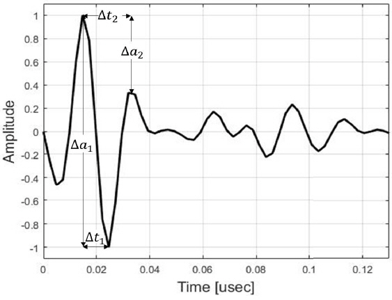
Waveform structure-based feature vector.

A study [5] shows the fusion of the feature vectors of the early-time and late-time regions extracted using the abovementioned method. The fusion method shows better performance than the methods using only the early-time feature vector or late-time feature vector. The early-time region feature vector based on the waveform structure is shown in Eq. (1):

The late-time region feature vector is the resonance frequency extracted by the EP-based CLEAN algorithm. In general, the response in the late-time domain of the radar signal can be expressed by Eq. (2) using the singularity expansion method (SEM).

In Eq. (2)s_m = σ_m + jω_m denotes m^th resonance frequency, a_m denotes the amplitude of the m^th resonance frequency, and φ_m denotes the phase. T_F is the time at which the late time region ends, and M is the number of resonance frequencies in the late time response. In this paper, we use the resonance frequency extracted by the EP-based CLEAN algorithm as the feature vector of the late time domain. The detailed EP-based CLEAN algorithm is as follows.

Step 1 is the initialization step. First, set m = 1. m is the repeated index value for the m^th resonance frequency extraction, and the measured or calculated late time response is defined as x_m(t_k) where k = 1,2,…, K, and K is the number of time samples.

Step 2 is the parameter extraction step. Here, we extract the values of a_m, σ_m, ω_m, and φ_m that minimize the cost function J_m as shown in Eq. (3) using the EP subroutine.

Here, when the sufficient number of generations has elapsed, the EP subroutine is terminated.

Step 3 is the component removal step. The component of the resonance frequency extracted in Step 2 is removed from x_m(t_k) to obtain the signal x_m+1(t_k) as shown in Eq. (4).

Step 4 is a termination confirmation step. After setting m = m + 1, if the desired M resonance frequencies are extracted, the algorithm is terminated. If not, the process returns to Step 2 and the process is repeated. As a result, the late-time EP-based CLEAN algorithm is a technique that iteratively extracts the parameters of Eq. (3) through the EP optimization technique. In this paper, parameters for two resonance frequencies are extracted according to these steps. The feature vectors of the late-time domain are as follows.

III. Feature Vector Fusion in Radar Structure

The radar structure can be divided into a monostatic structure, in which the transmitter and receiver are the same, and a bistatic structure, in which the transmitter and receiver are separated from each other. The general radar structure is a monostatic structure, in which various target recognition experiments are carried out. When an aircraft is designed with a stealth design, the back-scattering signal is reduced due to diffuse reflection. Therefore, in this case, the monostatic radar is difficult to detect; consequently, the use of bistatic radars is more effective. Previous studies on bistatic radars have been performed at Hannam University [12], which compared and analyzed the target classification performance at three bistatic angles (60°, 90°, and 150°). However, by considering only one radar structure, either monostatic or bistatic, enough information about the target cannot be utilized. Another previous study [8] showed improved target recognition performance by extracting scattering centers using fast Fourier transform (FFT)-based CLEAN [13] at each radar structure and combining them of monostatic and bistatic structures. In that study, experiments were performed on various bistatic angles, rather than one bistatic angle, to find the optimum bistatic angle with the best recognition performance.

IV. Two-Level Feature Fusion Method

This paper proposes a two-level feature vector fusion method. Here, a feature vector is fused in two steps. The first-level feature vector fuses an early-time region feature vector with a late-time region feature vector. The second-level feature vector fuses a monostatic feature vector with a bistatic feature vector. We performed experiments at three bistatic angles of 30°, 90°, and 150° to find the bistatic angle that exhibits the best target classification performance. The detailed two-level feature vector fusion method is as follows. The feature vector of the early-time region based on the waveform structure and the late-time region feature vector are fused as shown in Eq. (6):

Next, the first-level feature vectors obtained at monostatic and bistatic structure by Eq. (6) are fused once more as shown in Eq. (7):

The proposed two-level feature vector fusion method can consider monostatic and bistatic structures, and use the feature vectors of both the early-time and late-time regions. Simulations were performed at several bistatic angles. Fig. 2 shows a block diagram of the proposed method.

Fig. 2

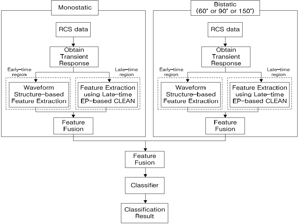
A block diagram of the two-level feature fusion method.

V. Simulation and Results

First, we used FEKO, a widely used electromagnetic analysis tool, for the target classification experiment. RCS was obtained for eight 3D full-scale targets (B-2, F-22, F-15, F-117, MIG-29, SU-27, J-20, T-50) similar to the actual size of target, and time-domain signals were obtained by inverse FFT. From these time-domain signals, feature vectors of the early-time and late-time regions were extracted. We used the method of moments (MoM) option for the calculation. The selected frequency range was the HF band (0.2–28 MHz), the frequency sampling point was 140 points with 0.2 MHz intervals, and the polarization was HH (horizontally transmitting, horizontally receiving) polarization. Elevation angles were fixed at 0°, assuming the target to be at a long distance, and the aspect angles were 0° to 180°, with 1° intervals, resulting in a total of 181 points. In addition, 50 Monte Carlo simulations were performed to increase the reliability of the experimental results.

In the target classification experiment, a neural network classifier is trained until a mean square error of 10⁻³ was reached. Data with SNR = 20 dB were used as the training data, while white Gaussian noise was added to the test data, with SNR = 5, 10, 15, and 20 dB. We also compared the target classification performance at three bistatic angles of 60°, 90°, and 150° to find the best bistatic angle showing the best performance. Prior to the two-level feature vector fusion, the target classification experiment was performed through the one-level feature vector fusion which uses only the first-level fusion step. The target classification results using the 8-dimensional feature vectors obtained through the one-level feature vector fusion were compared with those using the 16-dimensional feature vectors obtained through the two-level feature vector fusion. Fig. 3 show the comparison of target classification performance for each bistatic angle. The target classification percentage is the average of 50 Monte Carlo simulations, and the standard deviation was also shown as bar.

Fig. 3

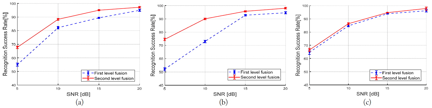
Comparison of classification performance when using the one-level feature vector fusion and the two-level feature vector fusion method. Three bistatic angles of 60° (a), 90° (b), and 150° (c).

As a result, at three bistatic angles of 60°, 90°, and 150°, target classification performance is improved when two-level feature vector fusion is used. At the bistatic angles of 60° and 90°, the lower SNR is, the more improved target classification performance is when the two-level feature vector fusion is used. At the bistatic angle of 150°, the difference between the one-level fusion and the two-level fusion is not big for all SNR.

Fig. 4 compares the results obtained by combining monostatic structures at bistatic angles of 60°, 90°, and 150°. When the second-level feature vector fusion was performed at the bistatic angle of 90°, the best classification performance was obtained in all SNR environments. This means that the optimum selection of the second-level feature vector fusion is the monostatic and the bistatic of 90°. Also, in the low-SNR environment, there was a big difference in the target classification according to the bistatic angles, but there was not a big difference in the high SNR environment according to the bistatic angles.

Fig. 4

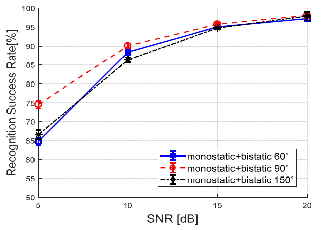
Comparison of classification performance when using three different second-level feature vector fusion.

As a result, both monostatic and bistatic radar structures were considered together with the feature vectors of both the early-time and late-time region. So, the target classification performance was improved by increasing the information of the target. Table 1 shows the confusion matrix at SNR = 20 dB and bistatic angle = 90°, which shows the best performance of the proposed method. The confusion matrix represents the relationship between the actual target and the classified target. The diagonal elements of the confusion matrix match the correct classification and other elements match the misclassification. In the confusion matrix shown in Table 1, the diagonal elements were close to 100% and the other elements of misclassification were very small. Therefore, we can overcome the problem of low resolution for the HF band radar by using the feature vector combining the resonance frequency and waveform structure.

Table 1

Confusion matrix of proposed method (bistatic angle = 90°, SNR = 20 dB)

VI. Conclusion

In this paper, we propose a two-level feature vector fusion method to improve the classification performance of the radar target. The proposed method combines the feature vectors of the early-time and late-time region and then combines them once more to the radar structure. We used the extracted parameters based on the waveform structure as the feature vector of the early-time region and the resonance frequency extracted by the late-time EP-based CLEAN algorithm as the feature vector of the late-time region. The feature vector based on the waveform structure and the resonance frequency can overcome the limitation of a narrow bandwidth in the HF band. To verify the performance improvement of the proposed method, we compared our method with the one-level feature vector fusion method, which fused only the feature vectors of the early-time region and the late-time region. The two-level fusion method is better than the one-level fusion method for all bistatic angles and all SNRs. We also do the simulation to find the optimum second-stage fusion combination for three bistatic angles. As a result, the best classification performance was obtained when the monostatic and bistatic 90° feature vectors were combined. Finally, we showed the confusion matrix of the proposed method. This result show that the all targets are well classified using the two-level feature vectors and misclassification is very small. Our method can be applied to the low frequency radar which can detect the low RCS targets such as stealth target or small missiles.

Article information Continued

References

Biography
In-Ha Kim received a B. S. degree in Electronics Engineering from Hannam University, in 2016. Currently, she is working toward an M.S. degree in Electronics engineering at Hannam University, Daejeon, Korea. Her research interests are radar signal processing and radar target classification.
Dae-Young Chae received a B.S. degree in Electronics Engineering from Sungkyunkwan University, Suwon, Korea in 2006 and an M.S. degree in Electrical and Electronics Engineering from Pohang University of Science and Technology (POSTECH), Pohang, Korea in 2008. Since 2008, he has been working at the Agency for Defense Development as a senior research engineer. His research interests include radar signal processing, RCS measurement, and NCTR.
In-Sik Choi received a B.S. degree in Electrical and Electronics Engineering from Kyungpook National University, Daegu, Korea in 1998 and M.S. and Ph.D. degrees in Electrical and Electronics Engineering from Pohang University of Science and Technology (POSTECH), Pohang, Korea in 2000 and 2003, respectively. From 2004 to 2007, he worked at the Agency for Defense Development as a senior research engineer. He is now a Professor in the Department of Electronics Engineering, Hannam University, Daejeon, Korea. His research interests include radar signal processing, RCS measurement and analysis, and EMI/EMC.