Dwell Time Optimization of Alert-Confirm Detection for Active Phased Array Radars
Article information
Abstract
Alert–confirm detection is a highly efficient method to improve phased array radar search performance. It comprises sequential detection in two steps: alert detection, in which a target is detected at a low detection threshold, and confirm detection, which is triggered by alert detection with a longer dwell time to minimize false alarms. This paper provides a design method for applying the alert–confirm detection to multifunctional radars. We find optimum dwell times and false alarm probabilities for each alert detection and confirm detection under the dual constraints of total false alarm probability and maximum allowable dwell time per position. These optimum values are expressed as a function of the mean new target appearance rate. The proposed alert–confirm detection increases the maximum detection range even with a shorter frame time than that of uniform scanning.
I. Introduction
Active electronically scanned antenna (AESA) technology improves airborne radar performance not only by reducing losses and increasing power efficiency with respect to conventional mechanical antenna but also through multifunctional aspects [1], such as fast exploration (steering), unpredictable scanning pattern, adaptive tracking rate independent of scan rate, and variable waveforms, among others [2]. This paper focuses on alert–confirm detection, the most significant technique to enhance AESA radar performance [3, 4].
Alert–confirm detection is also called energy-variant sequential detection, and it comprises a sequential detection procedure [5]. Conventional sequential detection procedures apply Wald’s sequential probability test [6] for radar detection. The likelihood ratio is calculated for each transmitted beam and compared with two thresholds. If the likelihood ratio exceeds the upper threshold, a target is declared; if the likelihood ratio drops below the lower threshold, no target is declared. If the likelihood ratio falls between the thresholds, an additional beam is transmitted and the process is repeated. Sequential testing yields an improvement of several decibels in radar sensitivity compared with uniform scanning detection. Alert-confirm detection is a simpler procedure. The likelihood ratio for each beam is compared with the lower threshold. If the threshold is exceeded in any resolution cell, a second beam is transmitted to the same direction, and the return likelihood ratio is compared with the higher threshold. A target is declared present when the thresholds are exceeded on both beams. Similar search efficiency to sequential probability ratio can be obtained by the optimum choice of the thresholds and beam energies [7].
The standard measure for detection performance of scanning radars against a target with a given cross-section is the detection range, in which either the per-scan or cumulative probability of detection has some specified value. Cumulative probability is defined as the probability that an approaching target has been detected at least once by the time it reaches a given range, and it can be increased by increasing either the per-scan detection probability or the scan rate [8]. However, the scan rate, which is the reciprocal of the frame time for uniform scanning radar, and the per-scan probability cannot be increased simultaneously. Therefore, determining whether to scan frequently with a low per-scan probability or infrequently with a high per-scan probability is a major surveillance radar design issue. Mallett and Brennan [9] provided the maximum detection range and frame time analytically as a function of the desired cumulative detection probability. They showed that although the average per-scan probability and the cumulative detection probability were similar for non-fluctuating targets, i.e., within approximately 2% optimum values, the accumulation gain was particularly significant for fluctuating targets. In airborne radars with dynamic targets and a cluttered environment, the per-scan probability of detection is an oscillation function of the target range [10]. Consequently, no single range and value pair for the per-scan probability of detection can provide a meaningful description of range performance. However, the cumulative detection probability, which monotonically increases, should yield a performance measure [11]. Alternatively, the detection rate, defined as the detection probability per unit time, has been proposed rather than the cumulative detection probability as the optimization goal [12, 13].
Brennan and Hill [7] proposed optimum parameters maximizing the range for a specified cumulative detection probability, including threshold levels and signal-to-noise ratios (SNRs) for each detection. They performed optimization under the constraint of a fixed false alarm probability per beam position. Frame time for calculating the cumulative detection probability was based on the total average SNR per beam position provided by the alert–confirm detection. The total average SNR was the sum of SNR at the alert detection and the average SNR at the confirm detection, in which the average SNR was calculated as the product of the false alarm probability of the alert detection and SNR at the confirm detection. They considered non-coherent integration processing as a loss.
This study provided a design method for applying the alert–confirm detection to multifunctional AESA radar, which performs surveillance and tracking concurrently.
We found optimal dwell times and false alarm probabilities to maximize the detection range under two constraints: fixed false alarm probability per beam position and maximum allowable time to perform the alert–confirm detection. The maximum allowable time was determined by target movement and the interval between alert detection and confirm detection. Non-coherent integration processing was considered in an explicit format, and the new target appearance rate was included when calculating the frame time, which had not been considered previously.
The performance of the designed alert–confirm detection was verified by the increased maximum range compared with that of uniform scanning detection.
The remainder of paper is organized as follows. Section II explains the basic formulas and constraints. Section III discusses in detail the optimization results and some parameters affecting performance. In addition, Monte Carlo simulation results are shown and compared with those from numerical calculation. Section IV summarizes and concludes the paper.
II. Basic Description
1. Alert–Confirm Detection
We assume that detection is to be processed by coherent and non-coherent integrations, as shown in Fig. 1. Dwell time can be expressed as
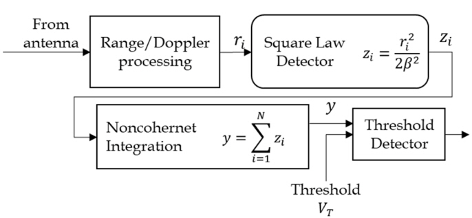
Simplified block diagram of non-coherent integration.
where T res is the time of the range bin, N rng is the number of range bins, N cn is the number of coherent integrations, N is the number of non-coherent integrations, and T coh is the coherent dwell time.
We assume that T coh is fixed and that the dwell time T d is dependent on N. The probability density function (PDF) of y is
where I N −1 is the modified Bessel function of order N–1, and R p = 2 × SNR [14]. The SNR is normally calculated by the radar range equation, which is
where
P̄ = average transmitted power
G = antenna gain
T d = dwell time
A e = effective aperture of the receiving antenna
σ = radar cross section (RCS)
A = amplitude related to σ (σ = A 2/2)
k = Boltzmann constant
T eff = effective noise temperature of the receiver
L = Loss factor
We use the Swerling I fluctuation model for airborne targets, where the amplitude is constant during one frame but varies independently from frame to frame [15]. The PDF of the amplitude A is described by a Rayleigh distribution expressed as follows:
where σ̄ is the average RCS.
As the Swerling I model requires the RCS to be constant during the integration or dwell time and vary between frames, RCS may or may not vary between alert detection and confirm detection depending on the interval between the detections. Therefore, we consider two cases of alert–confirm detection [7]: case 1 is quick confirmation (QC), in which the interval is short enough for RCS to be constant, and case 2 is late confirmation (LC), in which RCS varies because of the long interval. The overall detection probabilities for alert–confirm detection for cases 1 and 2 are expressed as
and
respectively, where
and i = 1 for alert detection and i = 2 for the confirm detection. The false alarm probability per cell can be expressed as
Therefore, the overall false alarm probability of the alert–confirm detection for m resolution cells is
[Constraint 1]
If the overall false alarm probability is given, the second threshold depends on the first. This overall false alarm probability is fixed to compare the performance with the uniform scanning detection.
For the alert–confirm detection, the confirm beam is transmitted in the same direction as the alert beam to ensure that the target remains in the angle of the radar beam. Therefore, the maximum allowable time per beam, T beam , for the alert–confirm detection is limited by target movement,
where T d 1 is the dwell time for alert detection, T d 2 is the dwell time for confirm detection, T in is the time between alert and confirm detections including the processing time, and T stay is the time that the target dwells in a beam direction. By substituting Eq. (1),
[Constraint 2]
where N 1 and N 2 are the numbers of non-coherent integrations in the alert and confirm detections, respectively.
When AESA radar performs surveillance and tracking concurrently, the frame time to calculate the cumulative detection probability can be expressed as
where ν is the mean new target appearance rate within the search volume, N beam is the number of search beams in a frame time, T track is the time for tracking the beams for multiple targets, and η̄ is the average number of unconfirmed search alarms per new target [16]. The second term, mP f 1 × N beam , represents the number of confirm beams from false alarms, and the third term, T s × ν(1 + η̄), is the number of confirm beams from the true target detection. T track can include any time required for tasks such as calibration, among others.
If T track is expressed as a ratio of the frame time, i.e.,
then the frame time in Eq. (12) is
where ω is the solid angle of the radar beam, and Ω is the solid angle of the search frame. As η̄ is dependent on T, T cannot be expressed in the closed form, and iteration is required to calculate T and η̄.
2. Cumulative Detection Probability
The cumulative detection probability at range R can be expressed as [9]
where P d (R′) is the per-scan probability at R′ for a given false alarm probability P f ; Δ = V c × T is the distance a target radially travels during a search frame, where V c is the target radial velocity, and l is the number of cumulations that equals the number of frames by the time the target reaches a given range from the initial detection range. The initial detection range is set large enough that the detection probability can be ignored.
To compare with the result of the alert–confirm detection, the detection range for the uniform scanning radar was calculated for P c = 0.85 as a function of the number of non-coherent integrations, N in Eq. (1). The scan area was defined as shown in Fig. 2 using a common 4 bar, ±60° scan raster. The bars were spaced 2.8° apart, and the number of beams in a bar was 30. The other parameters used in the simulation are listed in Table 1 [17].

Radar operation and the scan area.

Simulation parameters
Fig. 3 shows that the detection range R increases to its maximum as N increases from zero. In this interval, the effect of the increased per-scan detection probability exceeds that of the decreased scan rate. However, once R reaches its maximum, the effect of the scan rate is dominant, and the range decreases. The maximum range R 0 was 38.07 (NM) at N = 9. This result was verified by comparing with that in [9].
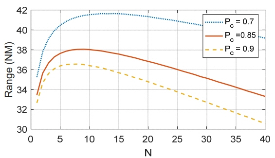
Range variation as dwell time (N) increases (Swerling I, P fa = 10−6).
III. Optimization for the Alert-Confirm Detection
1. Dwell Time Optimization
We performed the optimization for QC and LC cases discussed above. We assumed that the overall false alarm probability P fa = 10−6 and that the maximum allowable number N c = 50. Optimization aimed to find the parameters for P f 1, P f 2, N 1, and N 2 that maximize the detection range for a given cumulative detection probability (P c = 0.85). The overall optimization is summarized in Fig. 4.
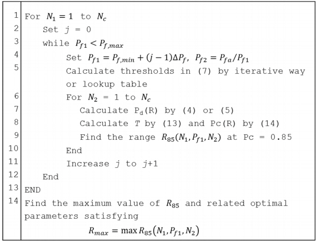
Summary of the optimization steps.
Fig. 5 shows the maximum detection range R as a function of N 1 when m = 32 and α = 0. N 1 increases the per-scan detection probability but decreases the scan rate. Therefore, as N 1 increases, R increases to its maximum point and then decreases monotonically. The change in R around the optimum is small. Fig. 6 shows the contour plots of R for N 2 and P f 1 at N 1 = 1 and at N 1 = 5. The change in R due to N 2 is also small when N 1 approaches its optimum (N 1 = 5).
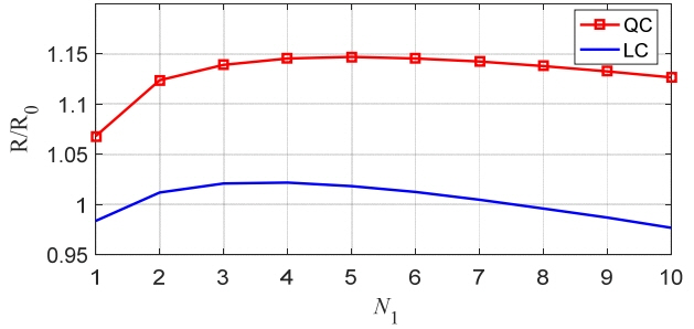
Maximum range for each N 1 at ν = 0.3 (m = 32, α = 0).

Contour plots for R/R 0 (QC, ν = 0.3 and α = 0): (a) N 1 = 1 and (b) N 1 = 5.
Optimization was repeated with changing the mean new target appearance rate, ν. If ν = 0, R/R 0 = 1.163 and 1.043 for QC and LC, respectively, as shown in Fig. 7. The increment is much larger for QC than for LC. In other words, QC, which keeps the target RCS constant between the alert and the confirm detection, has a significantly longer detection range than LC. Late confirmation even extends the detection range compared with the uniform scanning detection. The maximum range decreases as ν increases because more confirm detections are triggered. For LC, if ν is greater than 0.7, then the range drops below R 0. Fig. 8 shows the optimal values for N 1, N 2, and T. N 2 is larger than N 1 and the frame time is shorter than that of the uniform scanning detection. At ν = 0, T = 7 and 4.56 seconds for QC and LC, respectively, which are significantly less than T = 8.6 seconds for the uniform scanning. The total dwell time per beam position for QC is shorter than that for LC, e.g., N 1 + N 2 = 24 and 30, respectively, at ν = 0.6. If the RCS fluctuation time can be estimated in advance, the constraint Eq. (11) can be used for the QC condition. In this simulation, the constraint Eq. (10) appears only where ν = 0.2 – 0.3 in LC. Despite the shorter dwell time for QC, its frame time is longer than that of LC because its confirm detections by false alarms are greater than that of LC.

Increase in R/R 0 for each case.

Optimal numbers of non-coherent integrations and frame times: (a) optimal number N 1 for alert detection, (b) optimal number N 2 for confirm detection, and (c) optimal frame time.
The optimal false alarm probability does not change much with the new target appearance rate, as shown in Fig. 9. P f 1 = 10−3 for QC when ν is less than 0.5. Therefore, P f2 = 3.125 × 10⁻⁵ from (8). The false alarm probability for confirm detection is lesser than that for alert detection. That is, the threshold level for confirm detection is higher than that for alert detection.

Optimal false alarm probability for an alert detection.
From the above result, if ν is smaller than 0.3, the detection range is maximized when N 1 is 5, N 2 is 28, and P f 1 is 10−3 with quick confirmation.
Finally, we examined the effects of the number of resolution cells and the load of the tracking task. Figs. 10 and 11 show the effects of the number of resolution cells and the new target appearance rate. The maximum detection range decreases rapidly as m increases. The rate of the maximum range decrease is similar for all values of ν. Fig. 12 illustrates the range reduction as a function of the tracking load α, where the dashed line shows the range reduction for the uniform scanning detection. At α = 0.5, the maximum range decreases by 1 dB. For QC and LC, the reduction is 0.66 dB and 0.58 dB, respectively, which is less than that for the uniform scanning detection. LC shows the smallest reduction because it has the shortest frame time among the three cases.
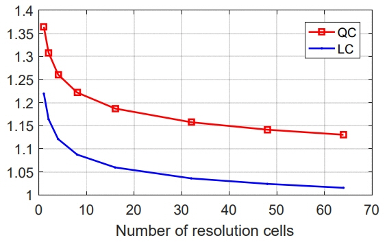
Effect of the number of resolution cells (ν = 0.1).

Effect of the number of resolution cells for varying ν (QC).
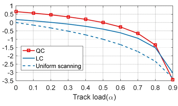
Performance degradation for the tracking load at ν = 0 and m = 32.
2. Monte Carlo Simulation
We also performed a Monte Carlo simulation to verify the above results using numerical calculations. This Monte Carlo model was developed to simulate the radar operation intuitively based on random signal generation. It can show the entire detection process if desired and simulate various scenarios including the detection strategies.
We generated more than 5,000 targets in 10,000 frames. The initial detection distance was set to 48 NM, and the target appearance rate ν was 0.3. The reflective signals from the targets were synthesized according to the RCS distribution as in Eq. (4), and the Gaussian random noise was added by SNR in Eq. (3). The detection range was defined as the range at which 85% of the targets were detected. The detection was decided by the false alarm probability or equivalently by the threshold level in Eq. (7).
Fig. 13 shows a typical screen capture during the simulation. Continuously changing beam positions and targets are displayed by different symbols.
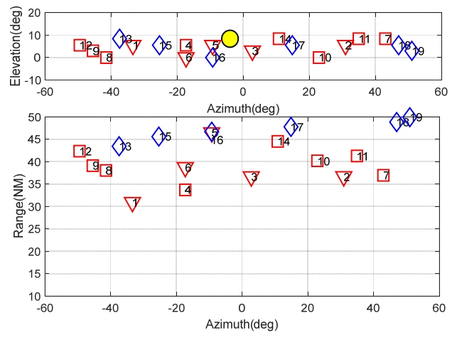
Example of a screen capture from the Monte Carlo simulation (
 : current beam position, ▽ : confirmed targets, □ : detected but not confirmed targets, ⋄ : undetected target).
The Monte Carlo simulation results were within 2% of the numerical calculation results, as shown in Fig. 14, for a typical example with ν = 0.3, N 1 = 5, and P fa 1 = 10−3. This model is useful to simulate complex scenarios or system diversity, including beam broadening at off-boresight angles, in which numerical calculation are difficult. Modifying the confirmation strategy (e.g., more than 1 out of 3 confirmation detections) is also possible to improve the detection range. This issue will be investigated in future research.
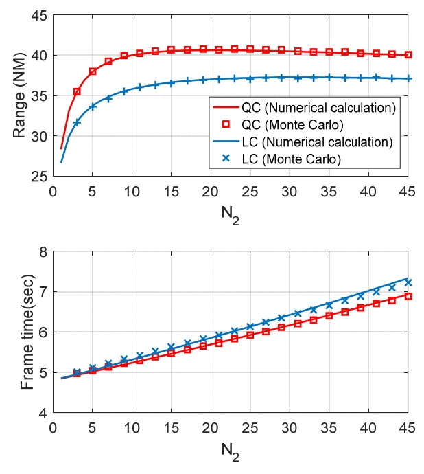
Comparison of the Monte Carlo simulation and numerical calculation results.
IV. Conclusion
Alert-confirm detection is one of the most significant techniques to improve the maximum detection range of surveillance radar. Although this strategy was proposed in the 1960s, the required beam agility and computational capability are now ready through the advanced AESA technology.
This study provides a design method for applying the alert–confirm detection to multifunctional AESA radar. We show the optimal parameters to maximize the detection range through a numerical method and the Monte Carlo simulation. In summary, the alert–confirm detection offers two advantages in comparison with the uniform scanning detection: improvement of the maximum detection range and reduced frame time. The reduced frame time improves the tracking performance of track-while-scan and active tracking.
We expect the variants of alert–confirm detection to further improve the performance of AESA radar, for example, having one alert and multiple confirmations. These variants are too complex to be written in an explicit form of equations. The Monte Carlo model can be useful to simulate these variants and various targets.
References
Biography
Eun Hee Kim received a Ph.D. degree in Mechanical Engineering from the Korea Advanced Institute of Science and Technology in 2004. She worked at LIGNEX1 for 6 years until September 2013. She is an associate professor at Sejong University. Her research interests are in radar signal processing and target recognition.

JoonYong Park received the M.S. degree in Electrical Engineering from Pohang University of Science & Technology (POSTECH) in 2016. He is a researcher at Agency for Defense Development. His research interests are in radar signal processing, estimation theory, AESA.
