Effects of Filling Material Roughness on Scattering from a Rectangular Groove

Article information

Abstract

I. Introduction

Given the importance of scattering by cavities in various applications, such as radar cross-section studies and non-destructive testing [1–3], considerable research has recently analyzed scattering from filled open cavities through different techniques [3–8]. In all these works, a cavity was assumed to be a very smooth surface, and the most important aspects examined were cavity shape as well as the accuracy and time efficiency of simulations.

The current research differs from previous studies in that it investigated the effects of filling material roughness on scattering from a rectangular groove given the important role that this property plays in scattering problems. From an electromagnetic point of view, describing a surface as smooth or rough depends on the frequency and incidence angle of waves. The calculation of scattering waves from rough surfaces is usually a difficult task, especially for complex geometric shapes and randomly distributed surfaces. In this regard, the small perturbation method has been suggested as an approach to modeling scattering waves from rough surfaces under low-frequency constraints [9]. Under high-frequency limitations, however, the Kirchhoff model is preferable in predicting the scattering of waves from a surface [10]. To expand approaches to modeling under these constraints, researchers developed the integral equation model (IEM), which covers all frequency intervals at high accuracy [11]. In [11], the authors introduced the IEM based on the electric field integral equation (FIE) and considered approximations of the phase of a Green’s function in the spectral domain. The author later enhanced his version of the IEM through some modifications [12]. Notwithstanding the value of these initiatives, however, little research has been devoted to the effects of filling material roughness on scattering from a rectangular cavity.

To address this gap, we inquired into the extent to which the weakly rough surface of a filled groove (such as a polished exterior with weak residual roughness) can change scattering signatures. To derive scattered fields, we used the FIE method in such a way that a closed-form integral equation for a rough surface was constructed and then solved via the method of moments (MoM), which uses the pulse basis function. The advantage of the FIE is that a problem with minimal mesh points can be solved in a way that enables the division of a rough surface into small elements. The challenge is that in commercial electromagnetic simulators for which complete numerical methods such as the MoM and FEM (finite element method) are used, the entire surface that surrounds a groove or its volume must be meshed. In these simulations, time efficiency is a problem. For example, in computing scattering waves from a small groove on a large object, the number of meshes and CPU time must be increased considerably. In this work, we assumed that the surfaces of two walls and the bottom portions of a rectangular groove and an infinite ground plane have a perfectly smooth surface and that the filling material has a weakly rough surface, thereby preventing maximum variations in the groove surface to exceed a few tenths of the wavelength of an incident wave and groove depth.

The rest of the paper is organized as follows. Section II describes some simplifying assumptions that were considered in the approximation of Green’s functions inside and outside the groove. In applying continuity in the tangential magnetic field to the rough surface, a logarithmic singular magnetic field integral equation (MFIE) was constructed for the equivalent magnetic current. Section III discusses the discretization of the MFIE with logarithmic singularity and its subsequent resolution via the MoM. We used a set of constant values for local points (pulse basis function) on the rough surface to approximate the equivalent magnetic current. Increasing the number of points employed enhances the accuracy of results. After the singularity was eliminated, the MFIE was converted into a system of linear equations. A solution of a linear system of N equations needs an operation count relative to N³. Section IV presents the comparison of the proposed technique with the FEM and MoM used in HFSS and FEKO. We also employed the proposed method to compare the scattering patterns of three typical cases: convex, concave, and smooth surfaces. The analysis of the results indicated that the roughness of a filling material can alter the scattering signature of a filled rectangular groove.

II. Problem Description

Let us assume that a two-dimensional filled rectangular groove is embedded on an infinite ground plane. The groove is created using three perfect conductor walls with a very smooth surface. The filling material has a continuous rough surface with an arbitrary profile l : y = f(x) (Fig. 1). An H-polarized incident plane wave illuminates the groove. By enforcing continuity in the tangential magnetic field on surface l, we derive

Fig. 1

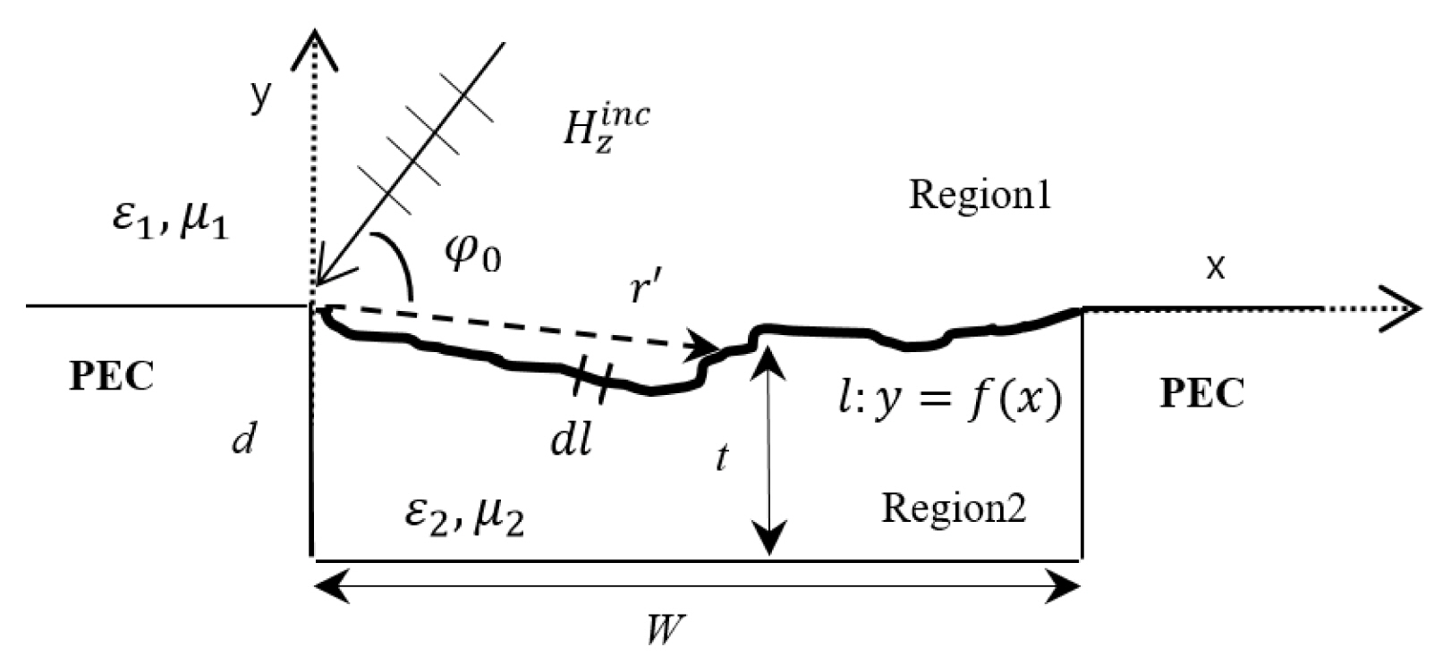
Geometry of a rectangular groove filled with a rough material ɛ₂, μ₂.

The sum of incident and reflected magnetic fields can be written as

where k₀ and ϕ₀ are the free space propagation constant and incidence angle, respectively. The z-component of the tangential magnetic field in regions 1 and 2 ( HzRegion1 and HzRegion2, respectively) on the rough surface are obtained as follows:

(b) Determining HzRegion2

We assumed that the maximum variations in the groove surface in terms of cavity depth and wavelength are small. We can therefore approximate the Green’s function G(r, r′) in the groove as

(4) G(r,r′)≈∑p=0∞ɛnWg(y≈0,y′) cos (pπxW) cos (pπx′W)

in which function g(y ≈ 0, y′) is estimated in the following manner:

(5) g(y≈0,y′)=g(f(x′))=1kp(x′) tan (kp(x′)t)

The variable k_p(x′) in Eq. (5) is given by

(6) kp(x′)=ω2ɛ0ɛrb(x′,f(x′))μ2-(pπw)2

where ɛ_rb(x′, f(x′)) is the effective relative dielectric permittivity of the filling material for the configuration shown in Fig. 2. This permittivity can be determined as follows [13]:

Fig. 2

A rectangular groove filled with a material with a weakly rough surface.

(7) ɛrb(x,y)=ɛrb(x,f(x))=ɛr2+∑i=1N(ɛr1-ɛr2)×(H (x-xi-Δ2)-H (x-xi+Δ2))×(H (f(x)-yi-hi2)-H (f(x)-yi+hi2))

in which H(. ) is the Heaviside function, N is the number of subdivision lengths Δ, the coordinate of the nth sector is at point (x_i, y_i), and its size is Δ, as determined on the basis of h_i.

With consideration for the Green’s function G(r, r′) in region 2, the HzRegion2 on the rough surface can be given by

(8) HzRegion2=-jkbYb∫0lM(r′)G(r,r′)dll:y=f(x)

Replacing Eqs. (3), (8), and (2) in Eq. (1) yields the following integral equation:

(9) 2ejk0((x-W2) cos ϕ0+y sin ϕ0)-k0Y02×∫0lM(r′)H0(2)(k0∣r-r′∣)dl=-jkbYb∫0lM(r′)G(r,r′)dl

Integral equation (9) is a Fredholm’s integral equation of the first kind and can be represented in the form below:

(10) B(x,y)=∫0lMz(x′,y′)K(x,x′,y,y′)dl

where K(x, x′, y, y′) and B(x, y) are defined as follows:

(11) K(x,x′,y,y′)=K(x,x′,f(x),f(x′))=K(x,x′)=k0Y02H0(2) (k0 (x-x′)2+(y-y′)2)-jkbYbG(x,x′)

(12) B(x,y)=B(x,f(x))=B(x)=2ejk0((x-W2) cos ϕ0+y sin ϕ0)

III. Solution of Integral Equation

Let us consider the rough surface l:y = f(x) illustrated in Fig. 1. Differential dl is defined as

Function N(x) is defined thus:

Substituting Eqs. (13) and (14) in Eq. (9) rearranges integral equation (9) as follows:

Numerous methods can be used to solve integral equation (15). To discretize it, we used the MoM, wherein function N(x) is approximated via the pulse basis function series with constant width Δ [8]. That is,

where x_n = nΔ – Δ/2 and N_n are the unknown coefficients of pulse expansion N(x′). When Eq. (16) in Eq. (15) is replaced and certain mathematical simplifications are performed, for each midpoint x_n, integral equation (15) becomes

in which

The singular integral in Eq. (17), which originates from the logarithmic singularity in Hankel function H0(2)(.), is given by

In accordance with the derivative definition, when x′ is close to x_m, we derive

The small argument approximation for the Hankel function in Eq. (21) is used in the following manner:

where β=k0∣xm-x′∣1+f′(x′)2, and γ = 1.78107 is Euler’s constant. Integrating singular integral (20) analytically yields

where e = 2.71828 is Nipper’s constant. In Eq. (17), taking N = M represents integral equation (15) in matrix form thus:

where N = [N₀, N₁, … , N_M] are the unknown coefficients that should be computed. B = [B(x₀), B(x₁), … , B(x_m)] is an excitation matrix, and matrix elements B_m are calculated as follows:

K_mn can be expressed as

Now, matrix N can be calculated through matrix inversion. After calculating unknown coefficients N_m, coefficients M_m are determined using Eq. (14), and then far-field waves and echo widths can be obtained using the formulas presented in [3]:

IV. Results

This section recounts the verification of the proposed method via the FEM and MoM solutions used in HFSS and FEKO. We carried out comparisons for the groove shown in Fig. 1 with convex (Fig. 3(b)) and concave (Fig. 3(a)) surfaces. Fig. 4(a) and 4(b) illustrate the effects of the angle of incidence on the backscattering echo widths of a filled groove with a concave surface (Fig. 3(a)) having the profile f(x) = 0.2x² – 0.4x and a filled groove with a convex surface (Fig. 3(b)) characterized by the profile f(x) = −0.2x² + 0.4x, respectively. The comparisons were conducted using FEM and MoM solutions to highlight the validity and accuracy of the proposed method (Fig. 4(a) and 4(b)). The results in Fig. 4 are in good agreement with the other numerical solutions. The echo widths are depicted in Fig. 4(a) and 4(b), and the echo width of a filled rectangular groove with a very smooth surface is shown in Fig. 5 to examine the difference between these echo widths. An analysis of the results presented in Fig. 5 indicated that so long as the incidence angle is greater than 80° (ϕ₀ > 80°), only a slight difference in echo widths occurs. As the incidence angle decreases, this difference increases. It also becomes more pronounced at grazing angles. A comparison of the diagrams displayed in Fig. 5 demonstrates that a rough surface can alter the levels and positions of dips.

Fig. 3

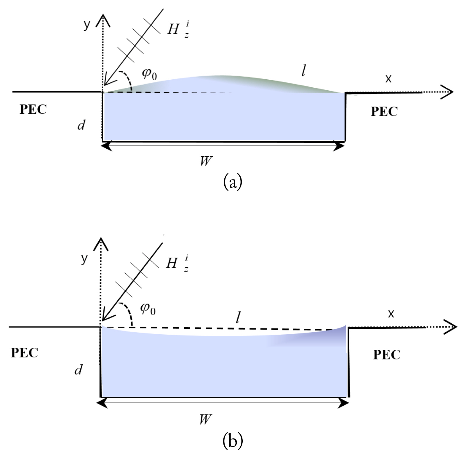
Geometry of a filled rectangular groove with (a) convex and (b) concave surfaces.

Fig. 4

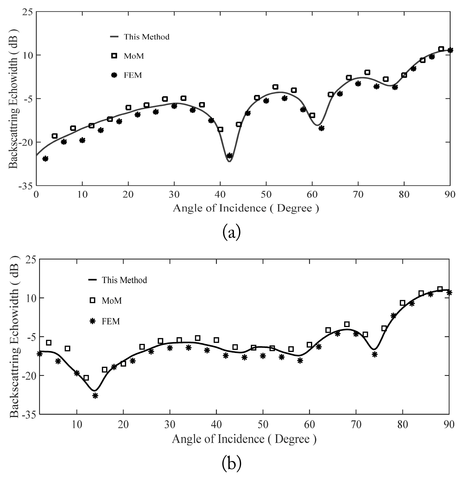
Backscattering echo widths of the rectangular groove with the rough surface shown in Fig. 3 for various incidence angles and the following conditions: w = 4λ, d = 1λ, ɛ_b = 2.5 – j0.2, μ_b = 1.8 – j0.1, as well as (a) convex surface (f(x) = 0.2x² – 0.4x) and (b) concave surface (f(x) = −0.2x² + 0.4x).

Fig. 5

Simultaneous display of the backscattering echo widths shown in Fig. 4.

We likewise used the proposed method to inquire into the effects of roughness on bistatic echo width. Taking the bistatic echo width pattern of the smooth surface as the reference, we can deduce from Fig. 6 that a rough surface affects bistatic echo width more strongly on the wave incidence side than on another region. In other words, back reflections change more frequently.

Fig. 6

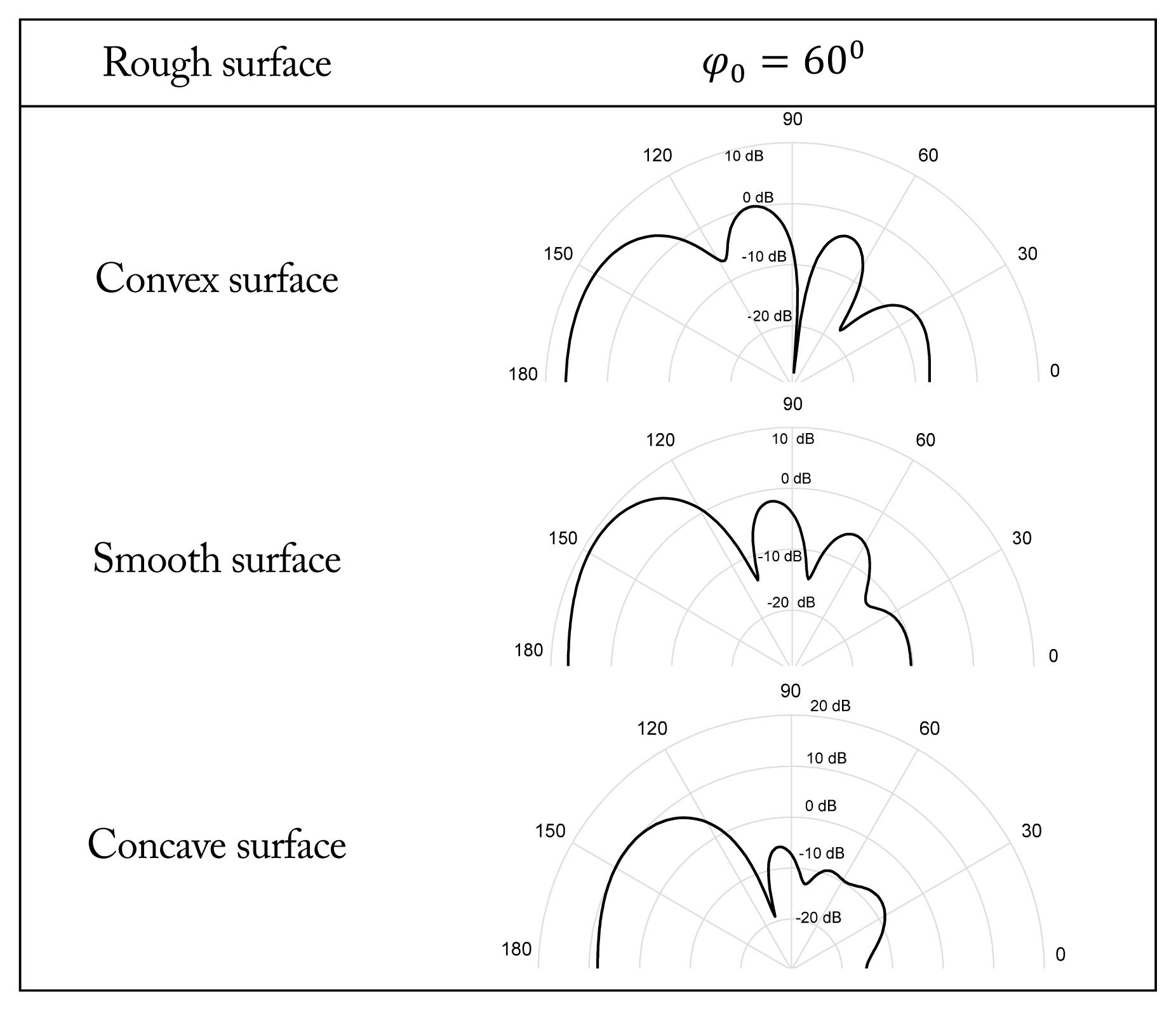
Bistatic echo width patterns for different rough surfaces of a filled rectangular groove at w = 4λ, d = 1λ, ɛ_b = 2.5 – j0.2, μ_b = 1.8 – j0.1, ϕ₀ = 60°.

Note, however, that as the gradient of surface equation (|f′(x)|) increases, the number of subdivisions N in Eqs. (7) and (16) should be augmented to derive accurate results. If such a gradient change rapidly at point x_m, or f′(x_m) ≈ ∞, the obtained findings would be invalid, and the method put forward in this work cannot be used.

Finally, the results suggested that a weak residual roughness of polished surfaces can alter monostatic and bistatic patterns. These changes are significant at some observation angles.

The solution of the problem described in this paper and its results can be used in radar cross-section reduction studies, nondestructive testing, and surface roughness testing applications.

V. Conclusion

The H-polarized scattering by a filled rectangular groove with a weakly rough surface embedded on an infinite ground plane was examined. We considered some appropriate approximations for Green’s functions to simplify and solve an integral equation on the groove surface. We employed this method to look into scattered waves from convex, concave, and smooth surfaces. The results showed that for incidence angles near the normal, backscattering echo widths are approximately equal. If an incidence angle decreases, the difference between backscattering echo widths increases. We also determined the bistatic patterns of the above-mentioned cases. The findings demonstrated that a weakly rough surface, such as a polished exterior with a weak residual roughness, can change scattering signatures considerably.

Article information Continued

References

Biography
Mehdi Bozorgi was born in Isfahan, Iran on September 4, 1977. In 2018, he joined Arak University in Arak, Iran where he is currently an assistant professor in the Department of Electrical Engineering. His current research interests include electromagnetic wave scattering, electromagnetic nondestructive testing, and optics.