Measurement of Analog Modulation Index with a Calibrated Radio Frequency Attenuator

Article information

J. Electromagn. Eng. Sci. 2021;21(2):87-94

Publication date (electronic) : 2020 April 30

doi : https://doi.org/10.26866/jees.2021.21.2.87

Chihyun Cho ¹^,, Hyunji Koo ¹, Jae-Yong Kwon ¹^,², Joo-Gwang Lee ¹, Tae-Weon Kang ¹

¹Group for Electromagnetic Metrology, Korea Research Institute of Standards and Science, Daejeon, Korea

²Science of Measurement Department, University of Science and Technology, Daejeon, Korea

^*Corresponding Author: Chihyun Cho (e-mail: chihyun.cho@kriss.re.kr)

Received 2020 July 20; Revised 2020 September 1; Accepted 2020 October 15.

Abstract

This paper presents a method for the accurate and traceable measurement of the analog modulation index. A calibrated step attenuator was used as the main apparatus because it has a higher dynamic range and lower uncertainty than a spectrum analyzer or an oscilloscope. In amplitude modulation (AM), the modulation index is obtained from the amplitude difference between the carrier and the first sideband, as in the conventional method. The resolution and calibration uncertainties of the step attenuator were propagated to the measurement uncertainty of the modulation index. The uncertainty produced by the impedance mismatch and repeatability was also included. For frequency modulation (FM) and phase modulation (PM), the modulation index, β, was estimated (with the step attenuator) from the spectrum of each sideband through the nonlinear fitting of the Bessel function. Thus, the uncertainty of the fitting process was added to the uncertainty of the measurement. The three modulations, AM, FM, and PM, exhibited an expanded uncertainty (approximately 95% confidence level, k = 2) of 0.372% for 50% nominal depth of the AM, 88.8 Hz for the peak frequency deviation of 10 kHz, and 0.88 mrad for a 0.1 radian modulation index, respectively.

Keywords: Amplitude Modulation; Frequency Modulation; Measurement Uncertainty; Metrology; Microwave Measurement; Modulation Index; Phase Modulation; Sensitivity Analysis

I. Introduction

Since the early 1900s, analog modulation has been used in wireless communication. It is still an important modulation scheme despite the extensive use of digital communications [1–3]. Analog modulation is one of the signal and pulse characteristics under the classification of the electricity and magnetism CMC (calibration and measurement capability) of the International Bureau of Weights and Measures. However, only a few National Measurement Institutes (NMIs) are listed. Moreover, there is no well-known measurement method with traceability.

Analog modulation can be measured in the frequency domain or the time domain [4–6]. In the preliminary work, we found that measuring the modulation index in the frequency domain is more effective than measurement in the time domain to reduce uncertainty. Thus, we measured the analog modulation index in the frequency domain in this study. Measuring the absolute power of a signal is usually important. Measuring the modulation index, however, requires a signal strength relative to the carrier, not the absolute power on each sideband.

In frequency modulation (FM) or phase modulation (PM), the modulation index is usually measured with the Bessel null technique. This method uses the characteristics of carrier or sideband signals have a value of zero when the modulation index achieves a specific value [5, 7]. Thus, the modulation index can only be measured at a specific value.

In this paper, we used a calibrated attenuator as the primary standard for the measurement of the modulation index. It is widely known that attenuators provide high accuracy and low uncertainty in the measurement of the relative signal strength. Moreover, the use of a calibrated attenuator readily makes the analog modulation index traceable to the measurement standard. In addition, we propose a method to measure the arbitrary FM and PM modulation indices through nonlinear fitting to overcome the limitation of the Bessel null technique. Finally, we analyze the measurement uncertainty of an analog modulation. To the best of our knowledge, this is the first comprehensive paper on analog modulation uncertainty analysis.

This paper is organized as follows. Section II describes the system for measuring the modulation index and the experimental evaluation of the effects of the impedance mismatch. Section III explains the measurement of the amplitude modulation (AM), FM, and PM modulation indices. Section IV explains the measurement of the relative amplitude of the sideband with the attenuator. Section V analyzes the uncertainty of each modulation index measurement, and Section VI concludes the paper.

II. Measurement Setup

1. Measurement Setup

Fig. 1(a) shows a block diagram and a photograph of the proposed measurement system for the analog modulation indices. The modulated signal generated by the device under test (DUT) was passed through the calibrated attenuator to the spectrum analyzer. The spectrum analyzer measured the strength of the carrier and sideband signals. Note that the spectrum analyzer had not yet been calibrated. The DUT and the spectrum analyzer were synchronized with 10 MHz, and each device was remotely controlled via a general purpose interface bus (GPIB, IEEE 488). We used a step attenuator with a resolution of 0.1 dB, which was calibrated at 0 dB to 100 dB [8].

Fig. 1

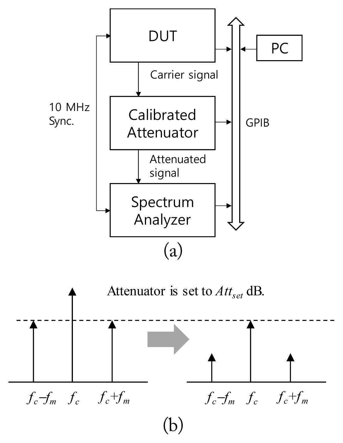
(a) Block diagram of the measurement system for measuring analog modulation index. The calibrated attenuator is used to correct the raw data measured by the spectrum analyzer. (b) Calibration procedure. First, the modulation signal is measured using the spectrum analyzer. Then, the attenuator is adjusted until the carrier signal is equal to the sideband signal.

2. Impedance Mismatch

Prior to measuring, we analyzed the effect of the impedance mismatch. The state of the impedance matching was adjusted by the insertion of an impedance stub tuner between the spectrum analyzer and the step attenuator (Fig. 2). The analog modulation index was measured by taking the relative amplitude difference between the carrier and sidebands (see a detailed explanation in Section III). Table 1 shows the measurement results. The absolute power of the carrier varied greatly on the basis of the status of the impedance stub tuner. The relative difference between the first sideband and the carrier, however, did not change regardless of the impedance matching status of the impedance tuner. Thus, the impedance mismatch did not significantly affect the analog modulation index measurement.

Fig. 2

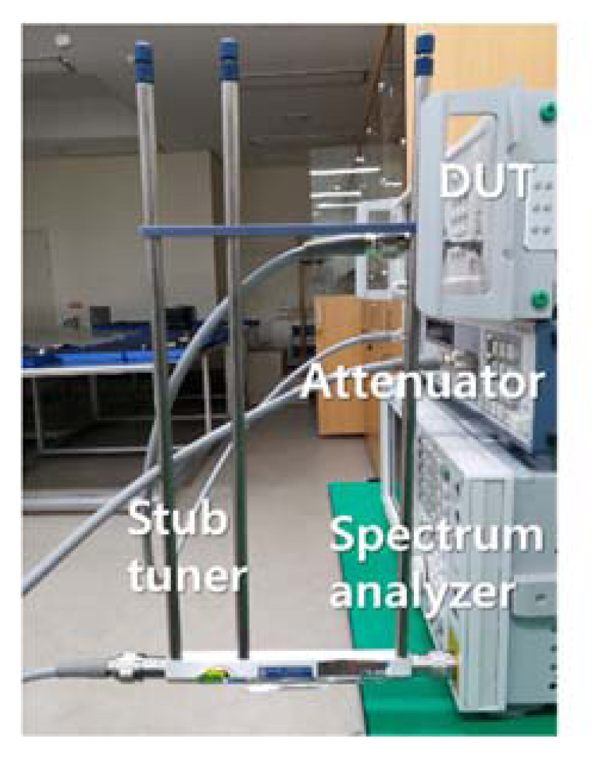
Measurement setup for the impedance mismatch effect between DUT and the measurement system. The impedance stub tuner is attached to the input port of the spectrum analyzer to produce arbitrary impedance matching status.

Table 1

Effect of the impedance mismatch

III. Modulation Index Measurement

1. Amplitude Modulation

AM changes the amplitude of the carrier, c(t), on the basis of the modulating signal or message, s(t). If s(t) is a continuous wave (CW), similar to that of the carrier, the AM signal, y(t), can be easily expressed as follows:

(1) c(t)=A cos(2πfct+φc)

(2) s(t)=Am cos(2πfmt+φm)

(3) y(t)=(1+s(t)A) c(t)=A cos(2πfct+φc)+12Am (cos (2π (fc+fm) t+φc+φm))+12Am (cos (2π (fc-fm) t+φc-φm))

where A is the amplitude of the carrier and m is the modulation index of AM. Thus, the amplitude of the sideband signal (f_c ± f_m) changes in proportion to the modulation index, and the modulation index is calculated as follows:

(4) m=2VSBVC=10ΔP+20 log10 (2)20

(5) ΔP=20 log10 (VSB/VC)

where V_C and V_SB are the amplitude of the carrier and sideband, respectively. The differences between the carrier and sideband signals on the dB scale are represented by ΔP, and it is easily obtained from the delta marker on the spectrum analyzer. In this paper, all the measured values were corrected with the calibrated attenuator for traceability to the measurement standard (details are provided in Section IV).

Fig. 3 shows the AM measurement results. For the DUT, the modulation index and the frequency of the modulating signal, f_m, were set to 50% and 50 kHz, respectively. Thus, the frequency interval between the carrier and sideband signals became 50 kHz. The nonlinear distortion was generated in the DUT because the large modulation index of 50% produced additional harmonics at f_c ± nf_m (n > 2). In theory, both of the first sidebands should have the same amplitude; however, they should exhibit asymmetric characteristics in the presence of FM distortion [9]. In this study, the average value of the two signals was used as the V_SB because the difference between them was very small, less than 0.005 dB. This value is counted as the standard uncertainty for the unbalanced sidebands, assuming a rectangular distribution of ±0.0025 dB.

Fig. 3

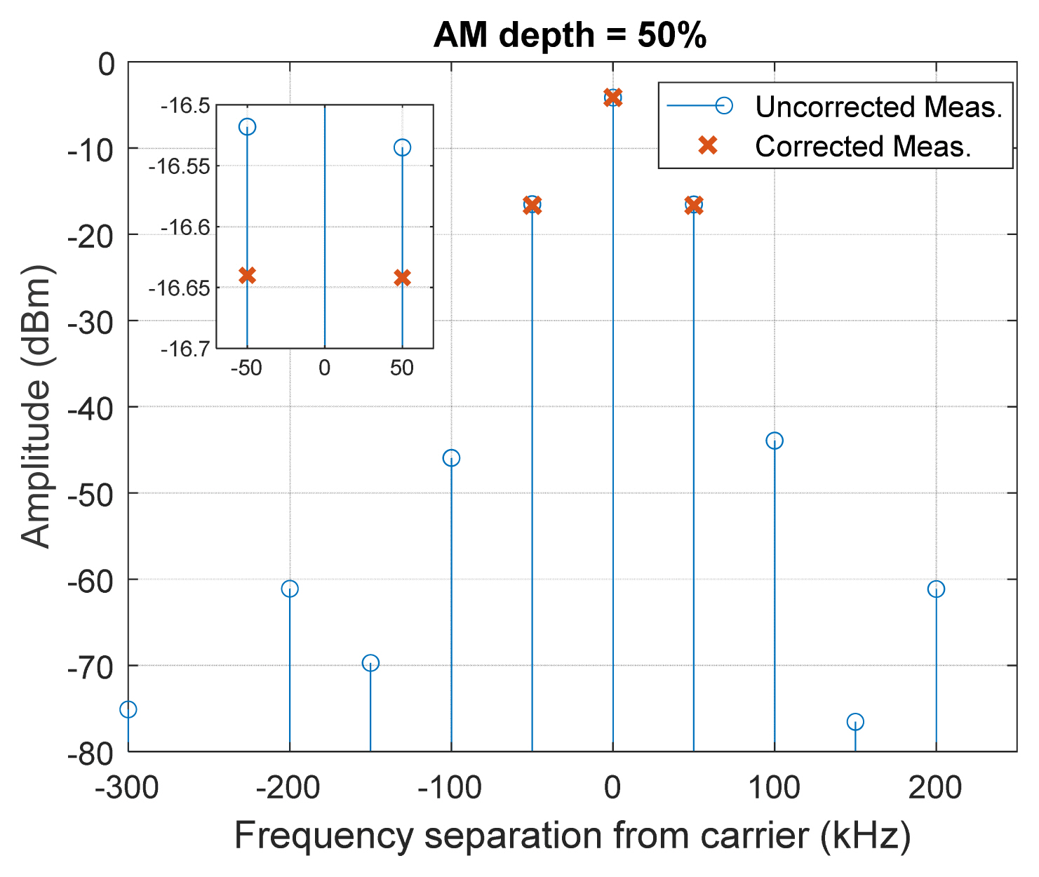
Measurement results for amplitude modulation (AM) with 50% of the AM depth where the carrier frequency is 500 MHz and the modulation repetition rate is 50 kHz. The uncorrected (raw measurement) and corrected (using the calibrated attenuator) amplitudes are represented with ‘—O’ and ‘X’, respectively.

2. Angle Modulation (FM and PM)

FM is expressed as (6), where Δf_p indicates the peak frequency deviation. Therefore, the changes in the frequency of y(t) depend on s(t). The amplitude, A, is time invariant:

(6) y(t)=A cos (2πfct+2πΔfp∫0ts(τ)dτ)

If s(t) is CW, as was the case for AM, (6) can be represented as follows:

(7) y(t)=A cos (2πfct+φc+Δfpfmsin(2πfmt+φm))=A cos (2πfct+φc+β sin(2πfmt+φm))

where β = Δf_p/f_m indicates the FM modulation index. Usually, the peak frequency deviation, Δf_p, is measured for a given frequency of the modulating signal, f_m. Eq. (7) also represents PM given that s(t) = cos(2πf_mt) causes a phase change on y(t). Thus, when s(t) is a sinusoidal function, the FM and PM have the same form, and they are commonly referred to as angle modulation. Mathematically, (7) can be expressed as the sum of the Bessel function of the first kind J as follows:

(8) A (∑k=0∞|Jk (β)|cos (2π(fc+kfm)t+φc+kφm)+∑k=-∞-1|Jk (β)|cos (2π(fc+kfm)t+φc+k(φm+π))

where k is the order of the sidebands. For example, when s(t) is a CW, the amplitude values of the carrier, first sideband, and second sideband are AJ₀(β), AJ₁(β), and AJ₂(β), respectively. As stated in previous section, the calculation of analog modulation index requires the relative difference between the carrier and each sideband. Therefore, the amplitude of carrier AJ₀(β) can be normalized to 1.

Then, the angle modulation index β can be estimated by minimizing the difference between the measurement and estimated values through nonlinear least squares fitting:

(9) ∑k=-nnymeas (k)ymeas (0)-|Jk (β)||J0 (β)|

Here y_meas(k) is the measured value of the k-th sideband. The nlinfit function in the MATLAB environment was applied as the estimator [10]. This is based on the Levenberg-Marquardt nonlinear least squares algorithm [11]. Nonlinear fitting problems often reach the local minima or slowly converge depending on the initial value. Robust results were obtained from the initial β, which is Δf_p divided by f_m (both are the values for the DUT setting).

Fig. 4 shows the measurement results. As was previously described, the number and shape of the generated sidebands depend on β. The fitted results (“x” marks) on the basis (9) agree well with the measured results (solid line). Estimation of β using 23 sideband measurements takes less than 0.05 seconds on an Intel Xeon E5 2.4 GHz CPU.

Fig. 4

Measurement results for phase modulation (PM) where the carrier frequency (f_c) is 500 MHz and the modulating signal (f_m) frequency is 100 kHz. (a) β = 0.1; (b) β = 3. The calibrated amplitude using the attenuator and the fitting result are represented with ‘—O’ and ‘X’, respectively.

IV. Calibration of Spectrum Analyzer with the Attenuator

The power of the frequency spectrum can usually be measured with a spectrum analyzer. As described in the previous section, the relative difference of the sideband signals, rather than the absolute power spectrum, was necessary to assess the measurement modulation index. Thus, for reducing measurement uncertainty and increasing precision, the calibrated attenuator is superior to the spectrum analyzer because of its higher dynamic range and lower uncertainty.

The difference between the carrier and sidebands, ΔP, as measured by a spectrum analyzer, can be corrected with a calibrated attenuator, as shown in Fig. 1(b). First, the modulation signal is measured using the spectrum analyzer. Then, the attenuator is adjusted until the carrier signal is equal to the sideband signal. Now the setting value of the attenuator Att_set can replace the uncalibrated ΔP. However, the reduced carrier signal may not be exactly the same as the power level of sidebands. Thus, the calibrated value can be calculated as follows:

(10) ΔPcorr=ΔPSA-Attset-ɛ

where ΔP_corr is the corrected difference on the basis of the attenuator. ΔP_SA is the raw measurement using the spectrum analyzer, and ɛ is the residual error that represents the power difference between the sidebands and the reduced carrier signal after the attenuator is set.

V. Uncertainty Analysis

1. Uncertainty of Amplitude Modulation Measurement

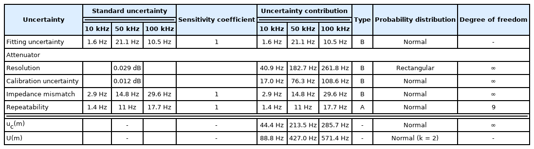
The measuring uncertainty of the AM modulation index is caused by the uncertainty introduced by the attenuator and the impedance mismatch between the DUT and the attenuator. The attenuator had a reading uncertainty of 0.1/(23) dB obtained from a resolution of 0.1 dB and a calibration uncertainty of 0.012 dB. If we actually correct the impedance mismatch by using the measured impedance values, the associated uncertainty will significantly increase due to the uncertainty of a vector network analyzer. To resolve this, we measured the difference the carrier and first sideband of the AM signal under an arbitrary matching condition in Table 1. To account for the uncertainty of the impedance mismatch for the scheme above, the standard deviation was obtained from the measured values in Table 1. Next, (4) was differentiated to propagate each uncertainty to the AM modulation index. The obtained sensitivity coefficient was log(10)×10ΔP+20 log 10(2)20/20. The coefficient was dependent on ΔP; thus, the large modulation index produced a large measurement uncertainty. Type A uncertainty was evaluated from 10 repeated measurements. The uncertainty budget is summarized in Table 2. The modulation index of 50% was measured, and the combined standard uncertainty, u_c(m) 0.186%, was obtained by taking the root sum of squares of the uncertainty contributions presented in Table 2. Since the effective degree of freedom is sufficiently large, the expanded uncertainty U(m) at approximately 95% confidence level is obtained by multiplying u_c(m) by 2.

Table 2

Uncertainty budget for AM modulation (f_m = 50 kHz and m = 50%)

2. Uncertainty for Frequency and Phase Modulation Measurement

Tables 3 and 4 show the uncertainty budget for FM and PM, respectively. In both cases, the angle modulation required additional uncertainty for estimating β from the measured amplitude of each sideband. Unfortunately, the fitting uncertainty for β could no longer be regarded as analytical. Instead, it was calculated from the residuals, which were calculated from the difference between the fitting model and measurements [12, 13]:

Table 3

Uncertainty budget for FM modulation (f_m = 100 kHz and Δf_p = 10 kHz, 50 kHz, 100 kHz)

Table 4

Uncertainty budget for PM modulation (f_m = 100 kHz and β = 0.1 rad, 1 rad, 3 rad)

(11) σresidual2=∑k=-nn|ymeas (k)ymeas (0)-|Jk (β)||J0 (β)||2/(l-p)

(12) σβ2=(∂σresidial∂β)2σresidual2

where l is the number of sidebands used in the measurement, including the carrier; thus, l is equal to 2n + 1. The number of unknown parameter β used in the fitting process, i.e., 1, is indicated by p. Therefore, the covariance for the fitting parameter σβ2 was calculated using (12) with the fitting residuals σresidual2. It must be noted that σ_β directly became the fitting uncertainty of β in PM. In the case of FM, the sensitivity coefficient was f_m because the peak frequency deviation was Δ f_p = f_mβ. Thus, the covariance of the peak frequency deviation σΔfp2 for FM was calculated as follows:

(13) σΔf2=(∂Δfp∂β)2 σβ2=fm2σβ2

The uncertainty of the attenuator could not be analytically propagated to the uncertainty of the FM and PM modulation indices because of the fitting process. Thus, Monte Carlo simulations were used to account for the uncertainty of the attenuator. The Monte Carlo simulations were performed separately for the reading and the calibration uncertainty of the attenuator because of their rectangular and normal distribution, respectively. The results are summarized in Tables 3 and 4. In addition, the impedance mismatch and repeatability uncertainties were accounted for in the same way as was done for AM. As shown in Fig. 2, the uncertainty of the impedance mismatch was evaluated by the insertion of the impedance tuner between the spectrum analyzer and the attenuator and the adjustment of the state of the tuner. The expanded uncertainty combining the above-described fitting uncertainty, attenuator uncertainty, impedance mismatch uncertainty, and repeatability was observed at 88.8 Hz to 571.4 Hz for FM (k = 2) and 0.88 mrad to 5.70 mrad (k = 2) for PM.

VI. Conclusion

We proposed an accurate method for measuring the analog modulation index. A calibrated attenuator was used to reduce measurement uncertainty and to ensure traceability. In the case of AM, the modulation index was measured by the power ratio of the first sideband and the carrier, as in the conventional method, and the measurement uncertainty was derived analytically. The 50% AM modulation index exhibited an expanded uncertainty (k = 2) of 0.372%. For FM and PM, the modulation index was measured through the nonlinear fitting of the Bessel function of the first kind by using the measured sidebands. Unlike the case for the Bessel null technique, the arbitrary modulation index could be measured. The measurement uncertainty obtained by the Monte Carlo simulation was 88.8 Hz for 10 kHz FM modulation and 0.88 mrad for 0.1 rad PM modulation. It is expected that the measurement uncertainty of analog modulation can be further improved with the application of an attenuator with a higher resolution.

Acknowledgments

This research was supported by Physical Metrology for National Strategic Needs, funded by the Korea Research Institute of Standards and Science (No. KRISS-2020-GP2020-0002).

Appendices

Appendix

The signal v_SA received by the spectrum analyzer is calculated as follows [14].

(14) vDUT=vSAh S21(1-ΓDUTS11-ΓSAS22-ΓDUTΓSA(S21S12-S11S22))

where v_DUT, Γ_DUT, Γ_SA, S_ij, and h are the output signal of the DUT, the reflection coefficient of the DUT, the reflection coefficient of the spectrum analyzer, S-parameters of the attenuator, and the frequency response of the spectrum analyzer, respectively. The frequency response of the sampler in most spectrum analyzers can be calibrated using [14–16]. Here, we assume h = 1 due to the narrow bandwidth of the analog modulation. In addition, when Γ_DUT, Γ_SA, S₁₁, and S₂₂ are negligibly small, the above formula is simplified as below.

vDUT=vSAS21

Note that most apparatuses have a small reflection coefficient. However, if the reflection coefficient is not so small that it is negligible, 10 dB attenuators with low reflection coefficients or tuners can be used as pads to reduce the mismatch between the DUT, the step attenuator, and the spectrum analyzer. Moreover, the output signal of the DUT can be calculated using (14) to include the mismatch effect. The corrected difference of the carrier and sidebands, ΔP_corr, can be calculated at a dB scale as follows:

(15) ΔPcorr=20 log10VDUTSBVDUTC=20 log10 (VSASBVSACS21CS21SB)=ΔPSA-Attset

where superscripts SB and C represent the sidebands and carrier, respectively.

References

1. Bahceci I, Khandani AK. Linear estimation of correlated data in wireless sensor networks with optimum power allocation and analog modulation. IEEE Transactions on Communications 56(7):1146–1156. 2008;

2. Guldemir H, Sengur A. Comparison of clustering algorithms for analog modulation classification. Expert Systems with Applications 30(4):642–649. 2006;

3. Carlsson C, Martinsson H, Schatz R, Halonen J, Larsson A. Analog modulation properties of oxide confined VCSELs at microwave frequencies. Journal of Lightwave Technology 20(9):1740–1749. 2002;

4. Humphreys DA, Harper MR, Roberts P. Preliminary results for a traceable amplitude modulation measurement technique using in-phase and quadrature referencing. In : Proceedings of 2007 International Waveform Diversity and Design Conference. Pisa, Italy; 2007; p. 145–149.

5. Keysight Technologies. Spectrum Analysis Amplitude and Frequency Modulation 2014. https://www.keysight.com/kr/ko/assets/7018-06742/application-notes/5954-9130.pdf .

6. Lee JG, Kim JH, Kang TW, Won SH, Lee DJ. RF peak power calibration of modulated signals. IEEE Transactions on Instrumentation and Measurement 60(7):2621–2626. 2011;

7. Roberts P. The challenges of precision analog modulation measurement. In : Proceedings of the Measurement Science Conference. Long Beach, CA; 2007;

8. Lee JG, Kim JH, Park JI, Kang UT. Uncertainty evaluation of a broadband attenuation standard. IEEE Transactions on Instrumentation and Measurement 54(2):705–708. 2005;

9. Matejka S. Accurate AM depth measurement in the presence of angle modulation. In : Proceedings of 2007 17th International Conference Radioelektronika. Brno, Czech Republic; 2007; p. 1–4.

10. Mathworks “MATLAB R 2019b” 2019. https://www.mathworks.com .

11. Seber GAF, Wild CJ. Nonlinear Regression Hoboken, NJ: John Wiley & Sons; 2003.

12. Cho C, Lee JG, Kang TW, Kang NW. Calibration and uncertainty analysis of sample-time error on high jitter of samplers. Journal of Electromagnetic Engineering and Science 18(3):169–174. 2018;

13. van de Geer S. Least squares estimation. Encyclopedia of Statistics in Behavioral Science Hoboken, NJ: John Wiley & Sons; 2005. p. 1041–1045.

14. Clement TS, Hale PD, Williams DF, Wang CM, Dienstfrey A, Keenan DA. Calibration of sampling oscilloscopes with high-speed photodiodes. IEEE Transactions on Microwave Theory and Techniques 54(8):3173–3181. 2006;

15. Dienstfrey A, Hale PD, Keenan DA, Clement TS, Williams DF. Minimum-phase calibration of sampling oscilloscopes. IEEE Transactions on Microwave Theory and Techniques 54(8):3197–3208. 2006;

16. Cho C, Koo H, Kwon JY, Lee JG. Uncertainty analysis for characterization of a commercial real-time oscilloscope using a calibrated pulse standard. IEEE Access 7:159724–159730. 2019;

Biography

Chihyun Cho received the B.S., M.S., and Ph.D. degrees in electronic and electrical engineering from Hongik University, Seoul, South Korea, in 2004, 2006, and 2009, respectively. From 2009 to 2012, he participated in the development of military communication systems at the Communication R&D Center, Samsung Thales, Seongnam, South Korea. Since 2012, he has worked with the Korea Research Institute of Standards and Science (KRISS), Daejeon, South Korea. In 2014, he was a guest researcher at the National Institute of Standards and Technology (NIST) in Boulder, CO, USA. He also served on the Presidential Advisory Council on Science and Technology (PACST) in Seoul, South Korea, from 2016 to 2017. His current research interests include microwave metrology, time domain measurement, and communication standards.

Hyunji Koo received the B.S. and Ph.D. degrees in electrical engineering from Korea Advanced Institute of Science and Technology (KAIST), Daejeon, Korea in 2008 and 2015, respectively. From March to August 2015, she was a Post-doctoral Research Fellow at the School of Electrical Engineering in KAIST. Since September 2015, she has been a Senior Research Scientist at the Center for Electromagnetic Standards in the Korea Research Institute of Standards and Science (KRISS), Daejeon, Korea. In 2018, she was a visiting researcher at the National Physical Laboratory (NPL), Teddington, UK. Her current research interests include characterization of on-wafer or PCB devices.

Jae-Yong Kwon received the B.S. degree in electronics from Kyungpook National University, Daegu, South Korea, in 1995, and M.S. and Ph.D. degrees in electrical engineering from the Korea Advanced Institute of Science and Technology, Daejeon, South Korea, in 1998 and 2002, respectively. He was a Visiting Scientist with the Department of High-Frequency and Semiconductor System Technologies, Technical University of Berlin, Berlin, Germany, and with the National Institute of Standards and Technology, Boulder, CO, USA, in 2001 and 2010, respectively. From 2002 to 2005, he was a Senior Research Engineer with the Devices and Materials Laboratory, LG Electronics Institute of Technology, Seoul, South Korea. Since 2005, he has been a Principal Research Scientist with the Division of Physical Metrology, Center for Electromagnetic Metrology, Korea Research Institute of Standards and Science, Daejeon. Since 2013, he has been a professor of the science of measurement with the University of Science and Technology, Daejeon. His current research interests include electromagnetic power, impedance, and antenna measurement.

Joo-Gwang Lee was born in South Korea in 1960. He received the B.S. degree in electronic engineering from Hanyang University, Seoul, South Korea, in 1984, and the M.S. and Ph.D. degrees from the Korea Advanced Institute of Science and Technology, Daejeon, South Korea, in 1994 and 2000, respectively. Since 1986, he has been with the Korea Research Institute of Standards and Science, Daejeon. His current research interests include radio-frequency and microwave measurements, time-domain metrology, and electromagnetic compatibility.

Tae-Weon Kang received the B.S. degree in electronics engineering from Kyungpook National University, Daegu, Korea, in 1988, and the M.S. and the Ph.D. degrees in electronic and electrical engineering from the Pohang University of Science and Technology, Pohang, Korea, in 1990 and 2001, respectively. He joined the Center for Electromagnetic Wave, Korea Research Institute of Standards and Science (KRISS), Daejeon, Korea, in 1990. In 2002, he spent a year as a visiting researcher under the Korea Science and Engineering Foundation for Post-Doctoral Fellowship Program with the George Green Institute for Electromagnetics Research, University of Nottingham, Nottingham, UK, where he was involved in measurement of absorbing performance of electromagnetic absorbers and a generalized transmission line modeling method. He has been involved in electromagnetic metrology and is currently a principal research scientist. His current research interests include electromagnetic metrology, such as electromagnetic power, noise, and antenna characteristics, and numerical modeling in electromagnetic compatibility.

Article information Continued

This is an Open-Access article distributed under the terms of the Creative Commons Attribution Non-Commercial License (http://creativecommons.org/licenses/by-nc/4.0) which permits unrestricted non-commercial use, distribution, and reproduction in any medium, provided the original work is properly cited.

Status	Power of carrier (dBm)	Difference between carrier and first sideband (dB)
A	−10	−12.482
B	−18	−12.483
C	−28	−12.467
D	−47	−12.471

Uncertainty	Standard uncertainty	Sensitivity coefficient	Uncertainty contribution	Type	Probability distribution	Degree of freedom
Attenuator
Resolution	0.029 dB	log(10)×10ΔP+20 log 10(2)20/20	0.167%	B	Rectangular	∞
Calibration uncertainty	0.012 dB	log(10)×10ΔP+20 log 10(2)20/20	0.069%	B	Normal	∞
Impedance mismatch	0.008 dB	log(10)×10ΔP+20 log 10(2)20/20	0.046%	B	Normal	∞
Imbalance of sidebands	0.002 dB	log(10)×10ΔP+20 log 10(2)20/20	0.012%	B	Rectangular	∞
Repeatability	0.003%	1	0.003%	A	Normal	9

u_c(m)	-	-	0.186%	-	Normal	∞
U(m)	-	-	0.372%	-	Normal (k = 2)	-

Uncertainty	Standard uncertainty			Sensitivity coefficient	Uncertainty contribution			Type	Probability distribution	Degree of freedom

	10 kHz	50 kHz	100 kHz		10 kHz	50 kHz	100 kHz
Fitting uncertainty	1.6 Hz	21.1 Hz	10.5 Hz	1	1.6 Hz	21.1 Hz	10.5 Hz	B	Normal	-
Attenuator
Resolution		0.029 dB			40.9 Hz	182.7 Hz	261.8 Hz	B	Rectangular	∞
Calibration uncertainty		0.012 dB			17.0 Hz	76.3 Hz	108.6 Hz	B	Normal	∞
Impedance mismatch	2.9 Hz	14.8 Hz	29.6 Hz	1	2.9 Hz	14.8 Hz	29.6 Hz	B	Normal	∞
Repeatability	1.4 Hz	11 Hz	17.7 Hz	1	1.4 Hz	11 Hz	17.7 Hz	A	Normal	9

u_c(m)		-		-	44.4 Hz	213.5 Hz	285.7 Hz	-	Normal	∞
U(m)		-		-	88.8 Hz	427.0 Hz	571.4 Hz	-	Normal (k = 2)	-

Uncertainty	Standard uncertainty			Sensitivity coefficient	Uncertainty contribution			Type	Probability distribution	Degree of freedom

	0.1 rad	1 rad	3 rad		0.1 rad	1 rad	3 rad
Fitting uncertainty	0.03 mrad	0.34 mrad	0.11 mrad	1	0.03 mrad	0.26 mrad	0.11 mrad	B	-	-
Attenuator
Resolution		0.029 dB		-	0.40 mrad	2.63 mrad	1.43 mrad	B	Rectangular	∞
Calibration uncertainty		0.012 dB		-	0.17 mrad	1.09 mrad	0.60 mrad	B	Normal	∞
Impedance mismatch	0.07 mrad	0.21 mrad	0.21 mrad	1	0.07 mrad	0.21 mrad	0.21 mrad	B	Normal	∞
Repeatability	0.03 mrad	0.15 mrad	0.15 mrad	1	0.03 mrad	0.15 mrad	0.15 mrad	A	Normal	9

u_c(m)		-		-	0.44 mrad	2.85 mrad	1.56 mrad	-	Normal	∞
U(m)		-		-	0.88 mrad	5.70 mrad	3.12 mrad	-	Normal (k = 2)	-