


I. Introduction
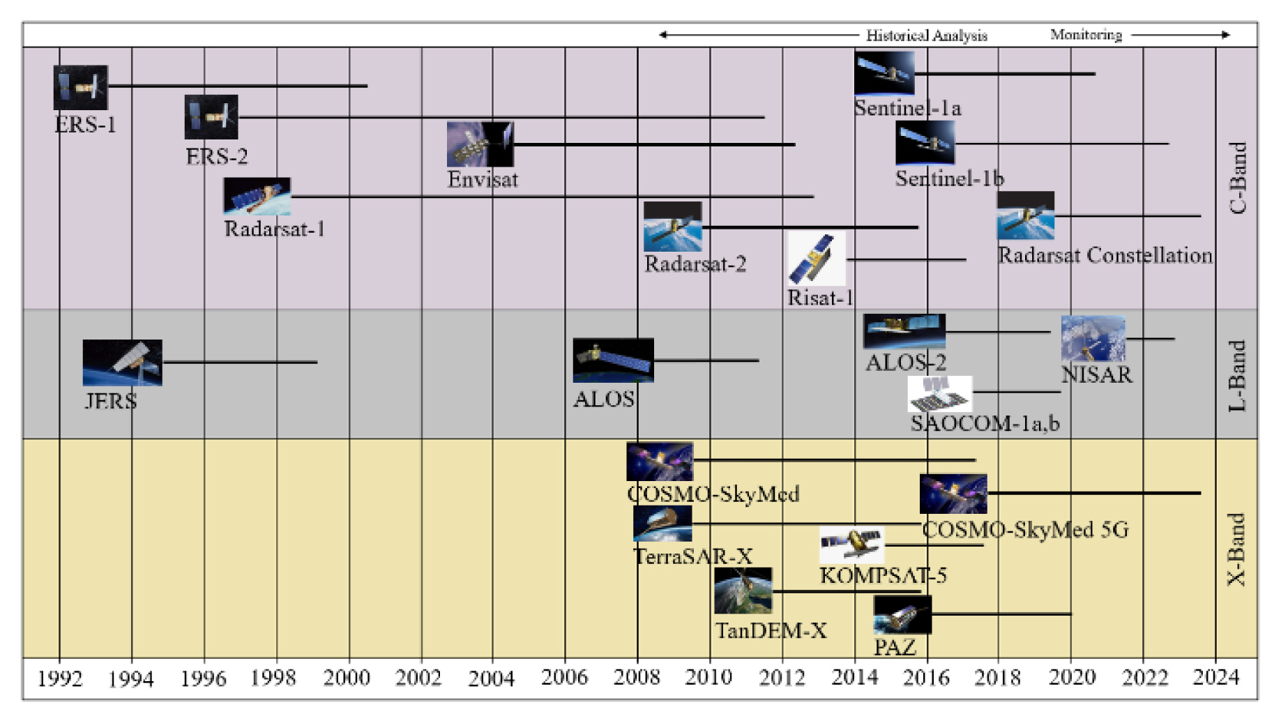
As global warming progresses, the Earth is rapidly changing, with polar glaciers thinning and sea levels rising. To detect these changes and predict the rate of global warming, it is essential to continuously observe the ocean. In 1978, the National Aeronautics and Space Administration (NASA) launched the world’s first Earth-orbiting satellite called “SEASAT”. SEASAT is equipped with L-band SAR for remotely acquiring images of the ocean [1]. Since high frequencies are advantageous for precise observation, the operating frequency of satellite SAR has been gradually increased. Fig. 1 shows the operating frequencies of synthetic aperture radar (SAR) satellites that have been or will be launched worldwide [2]. It can be seen that the operating frequencies of SAR satellites are upper limited to the X-band frequency. When designing an SAR system, the higher the operating frequency, the easier it is for the antenna to be miniaturized, which improves the azimuth resolution of SAR images [3].
Considering that the radar bandwidth is just a small fraction of the operating frequency and range resolution is inversely proportional to signal bandwidth, a high operating frequency also helps to improve the range resolution of SAR images. Despite these facts, the frequency of the satellite SAR is limited to the X-band frequency due to the upper limit of the PRF (pulse repetition frequency) value of the SAR system. The azimuth bandwidth of the target is well known as the following [3]:
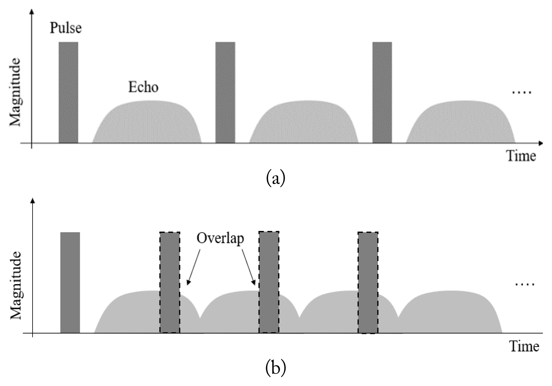
where Δfaz is the azimuth bandwidth, Vs is the velocity of SAR platform, θsq is the squint angle, λ is the radar wavelength, θbw is the azimuth beamwidth of SAR antenna, and La is the azimuth length of SAR antenna. Even though the λ term disappears in the azimuth bandwidth equation, La becomes shorter as the frequency increases to keep θbw at a reasonable value. The antenna beamwidth should be thin enough to ensure high antenna gain to compensate for long distances between the satellite and the target. At the same time, the beamwidth should be wide enough to obtain a reasonable length of range swath. Therefore, the ratio of radar wavelength and antenna length should be fixed to some extent. In order words, the shorter the radar wavelength, the shorter the antenna length and the wider the Doppler bandwidth. Meanwhile, in order to prevent aliasing that causes ghost effects in the SAR image, the PRF should be larger than the Doppler bandwidth to satisfy the Nyquist sampling rate. However, the PRF cannot be arbitrarily large since it is necessary to secure a sufficient pulse interval for a sufficient size of receiving window.
As represented in Fig. 2, if the PRF is too high, there is not enough room to receive the reflected signal from the range swath width. For automobile and aircraft SAR, even with the operating frequency of Ku-band or Ka-band, the azimuth bandwidth can be kept small because the platform is slow enough. However, for satellite SAR, the platform is tens or hundreds of times faster than automobile or aircraft cases, so frequencies beyond the X-band cannot be used.
For the next generation of the satellite SAR to advance to higher frequencies, we propose a low-complexity SAR algorithm that forms images of the ocean using satellite altimeter data. We have used data from CryoSat-2, which is a satellite altimeter developed by the European Space Agency (ESA). This paper is organized as follows. In Section II, an explanation about the burst mode pulse transmission and the data acquisition geometry of SAR altimeter is given, which is essential for the proposed algorithm. Section III introduces the proposed algorithm and presents a comparison with the existing algorithms. An example of ocean image results from CryoSat-2 data is also given. In Section IV, point target simulations and analysis are performed and some quantitative results are provided to verify the proposed algorithm. Finally, the conclusion of this paper is given in Section V.
II. Burst Mode Pulse Transmission and Data Acquisition Geometry of SAR Altimeter
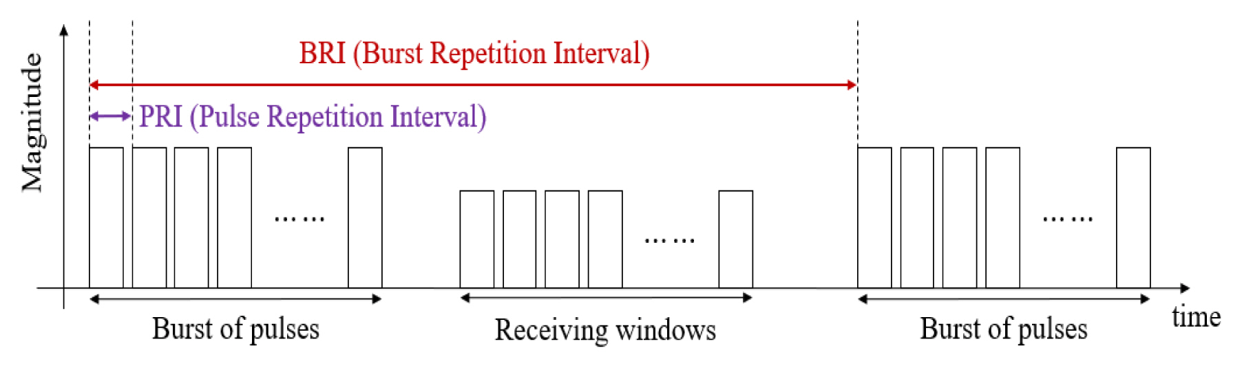
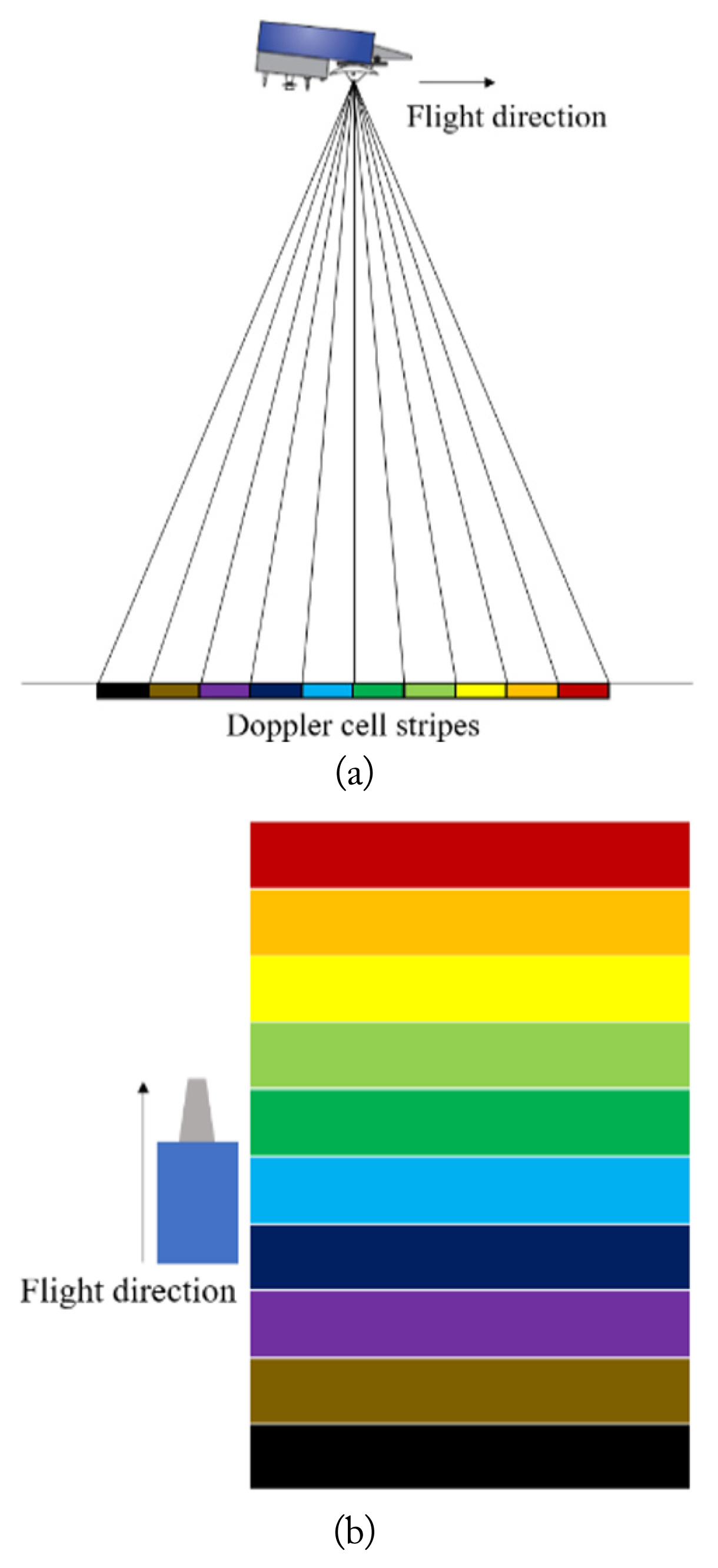
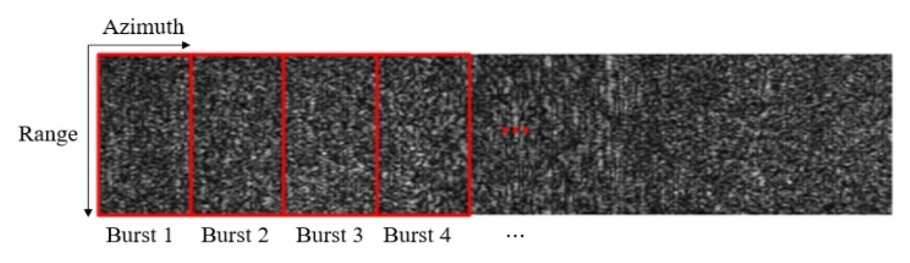
As mentioned in Section I, the frequency of the satellite SAR is limited to X-band frequency due to the upper limit of the PRF value. However, CryoSat-2 (Ku-band) is free from this problem because it utilizes a modified pulse transmission technique called “Burst mode”, as shown in Fig. 3. For CryoSat-2, one burst consists of 64 pulses, and the interval between adjacent bursts is defined as the burst repetition interval (BRI). These 64 pulses are emitted explosively with very high PRF to satisfy the Nyquist sampling rate. The reflected echoes are received through 64 receiving windows. Corresponding to these 64 pulses, the radar beam is divided into 64 narrow sub-beams in the along-track (azimuth) direction, and therefore, the illuminated area is also divided into 64 very narrow stripes of cross-range space, as illustrated in Fig. 4(a). CryoSat-2’s data acquisition geometry resembles that of real-aperture radar in that it utilizes narrow azimuth beamwidth and each pulse observes a different stripe. Therefore, an azimuth compression process is not required because there is no phase history in the azimuth direction (low-complexity). However, a sample stripe cell is continuously detected by each burst while the sample is in the beam-illuminated area; therefore, the synthetic aperture concept can be applied, as illustrated in Fig. 5. Ls is the synthetic aperture length. As the satellite moves along the track from position A to C, the sample stripe cell is detected by each burst with different Doppler frequencies (i.e., different look angle). However, since BRI is a fairly long value of 11.7 ms, each reflected echo is uncorrelated in terms of phase.
Before explaining the algorithm, the actual data acquisition geometry of CryoSat-2 must be clarified. Since the original function of CryoSat-2 is an altimeter, the data acquisition geometry follows that of nadir-looking radar, as illustrated in Fig. 4. In this case, it is not possible to discriminate points on the left and on the right of the sensor placed at the same range, and therefore it is not possible to obtain an SAR image. However, since the CryoSat-2 satellite antenna is somewhat tilted in the cross-track (range) direction, actual data acquisition geometry follows that of side-looking (near-nadir) radar [4], as illustrated in Fig. 6. The CryoSat-2 data we used were obtained when the antenna was tilted about 1.1° in the cross-track direction. Considering that the antenna beamwidth in the range direction is about 1.2° in Table 1, there is no need to worry about the left/right range ambiguity.
III. Ocean Image Formation Algorithm Using Satellite Altimeter Data
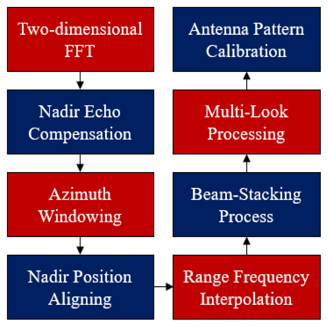
Table 1 shows main system specifications of the CryoSat-2. It is notable that the operating frequency is Ku-Band (13.575 GHz). The block diagram of the proposed ocean image formation algorithm is shown in Figs. 7 and 8 shows raw data of CryoSat-2. Each red box represents received raw data from a single burst. A single burst structure consists of 64 columns corresponding to 64 complex time domain echoes.
1. Two-dimensional Fourier Transform
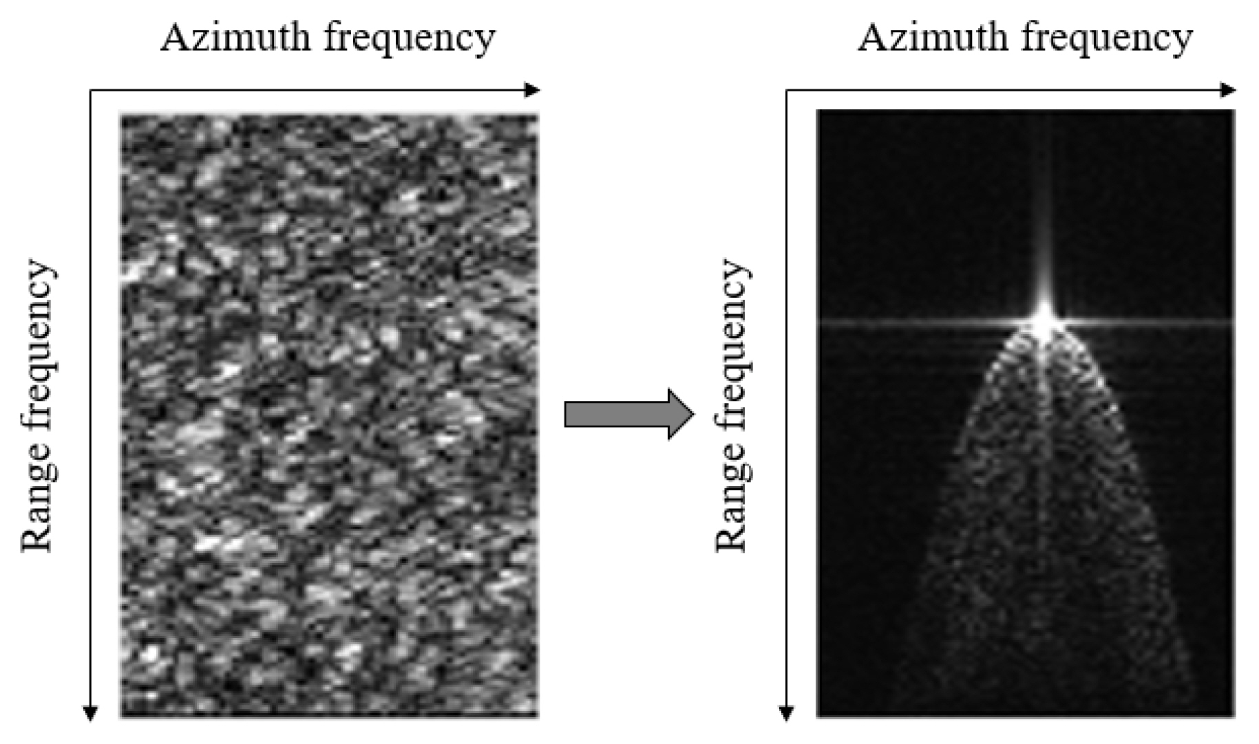
Transmitted pulses are linear frequency modulated continuous wave (FMCW), and the received echoes are de-ramped at the radar receiver. That is, the data in the range direction is composed of many continuous waves with frequencies proportional to the satellite-to-sample ranges. Therefore, range compression is implemented by the range Fourier transform [6]. Meanwhile, the azimuth direction of each burst consists of 64 received pulses. Since these 64 reflected echoes are obtained from successive pulses with explosive PRF and slightly different look angles, the data can be separated into each echo corresponding to Doppler cell stripes by azimuth Fourier transform. Fig. 9 shows the two-dimensional Fourier transform result of a single burst. It has distinct features in that the central beam receives the reflected echo with the greatest power at the nearest distance and the wider the angle between the Doppler beam and the central beam, the longer it takes for the reflected echo to be received and the less the received power. These are natural phenomena since the central beam observes the surface in a near-nadir direction with the shortest distance to the surface and the least power attenuation.
Another distinct feature is that the signal is detected in the same range for every Doppler stripe cell. This weird horizontal line is near-nadir clutter caused by the antenna side lobe ambiguity effect [7]. The echo from near-nadir sneaks through the antenna side lobe and aliases the signal that is received from the main lobe. Therefore, the near-nadir echoes exist at the same time (same range) in all Doppler beams in a single burst.
2. Nadir Echo Compensation
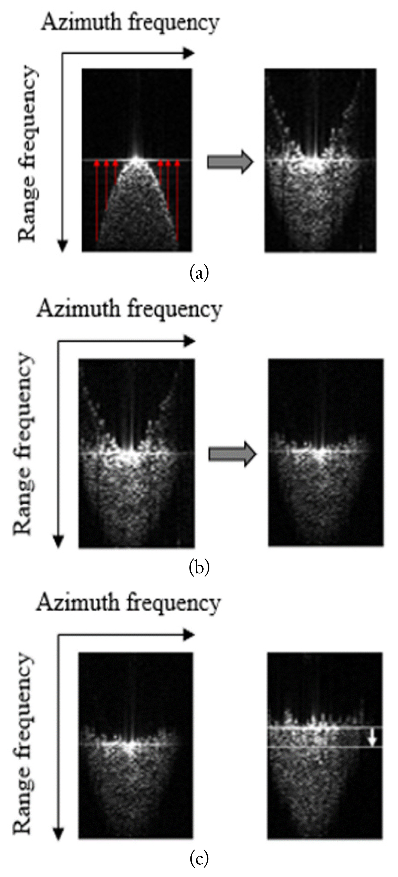
Fundamentally, SAR imaging is the process of determining the ground reflectivity of the observed area by mapping the received signal to the correct location. Since CryoSat-2 is actually a side-looking radar, it is possible to obtain an image by finding out from which exact sample the received signal originates. In fact, from the data acquisition geometry and specification of the SAR system, the slant range of closest approach and, therefore, the number of range bins of every single ground-sample can be calculated, although the task is very tedious. However, by using Nadir Echo Compensation (NEC), slant range correction is possible without such a tedious task. In each Doppler beam, the range bin number where the nadir (actually, near-nadir) echo is present is the position where the first return of echo should be located. This is because these points will be nadir points of the satellite’s orbit. Therefore, by using the nadir echo line shown in Section I, range misalignment can be fixed in every single burst. This is the core idea behind the NEC. This process is illustrated in Fig. 10(a). NEC is similar in effect to the range correction process used in other existing SAR algorithms in that it compensates for the range misalignment between adjacent azimuth sample stripes. The advantage of NEC over other range correction processes is that it is simple and much faster because it doesn’t need an interpolation process that requires a lot of computational loads.
3. Azimuth Windowing
After NEC is finished, nadir echoes that are no longer needed are removed by applying a window along the azimuth direction at raw data level, as shown in Fig. 10(b). Since windowing suppresses only the side lobe effect, nadir echo due to the antenna main lobe still remains. This remaining nadir echo will additionally be used in “nadir position aligning (NPA)” as a reference point that represents the nadir point of the satellite.
4. Nadir Position Aligning
While the NEC corrects range misalignments within a single burst, the NPA corrects range misalignments between adjacent bursts. If there is a drastic change in the nadir point of the satellite between adjacent bursts, the drastically changed nadir point of satellite is rearranged to the reference point of the previous burst. This process corrects the nadir line to match with the ground track of the satellite. The NPA is illustrated in Fig 10(c).
5. Range Frequency Interpolation
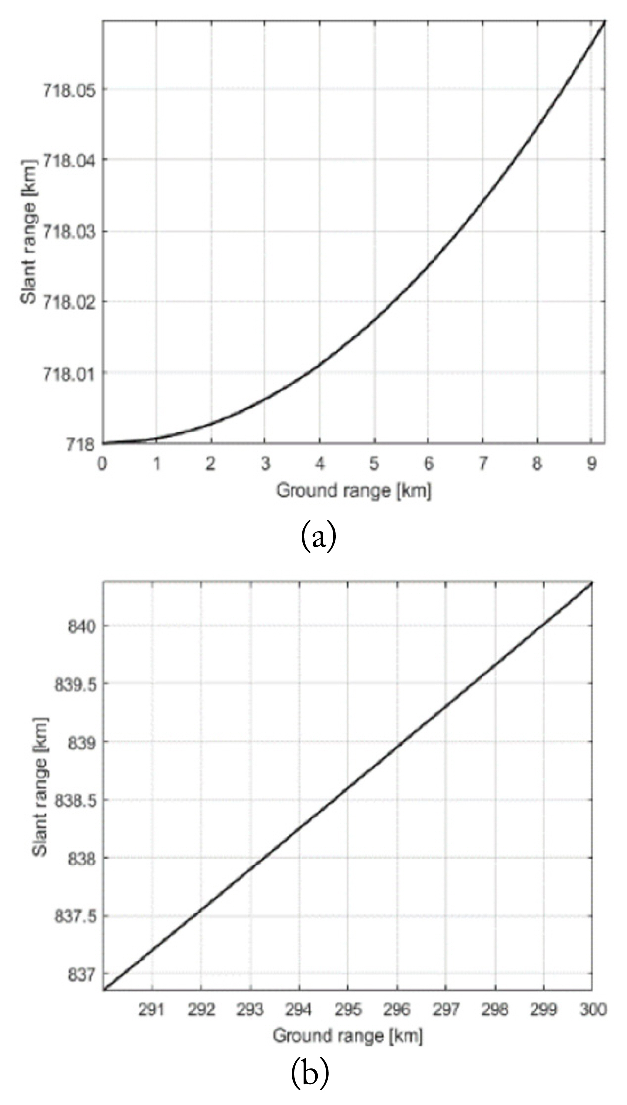
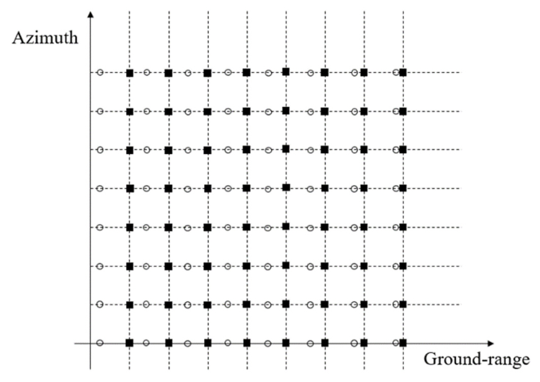
In general image SAR satellites, the look angle is wide enough that the relationship between the slant range and the ground range is approximately linear, as shown in Fig. 11(b). However, in the case of CryoSat-2, the look angle is so narrow that the relationship between the slant range and the ground range is nonlinear, as shown in Fig. 11(a). Due to this nonlinearity, the resultant ground range samples become unevenly spaced. In Fig. 12, the white circles represent given unevenly spaced data points, and the black squares represent the evenly spaced data points to be found. Therefore, interpolation from unevenly spaced data was performed to provide evenly spaced samples in the ground range domain. We named this process “range frequency interpolation” since it is performed on the range frequency domain.
6. Beam-Stacking Process
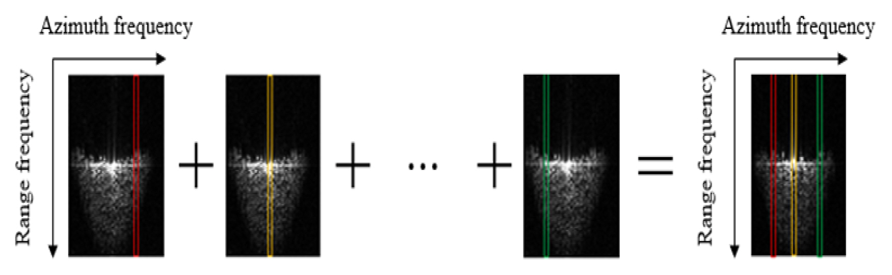
As described in Section II and Fig. 5, there are many independent Doppler beams that observe a particular sample stripe cell in the synthesized antenna. These independent Doppler beams point a sample stripe cell at different look angles from different bursts. Collecting these independent Doppler beams into a single stack is called the beam-stacking process. Fig. 13 visually illustrates the beam-stacking process. In the beam-stacked data, the x-axis represents the beam order that observes the sample stripe cell.
7. Multi-Look Process
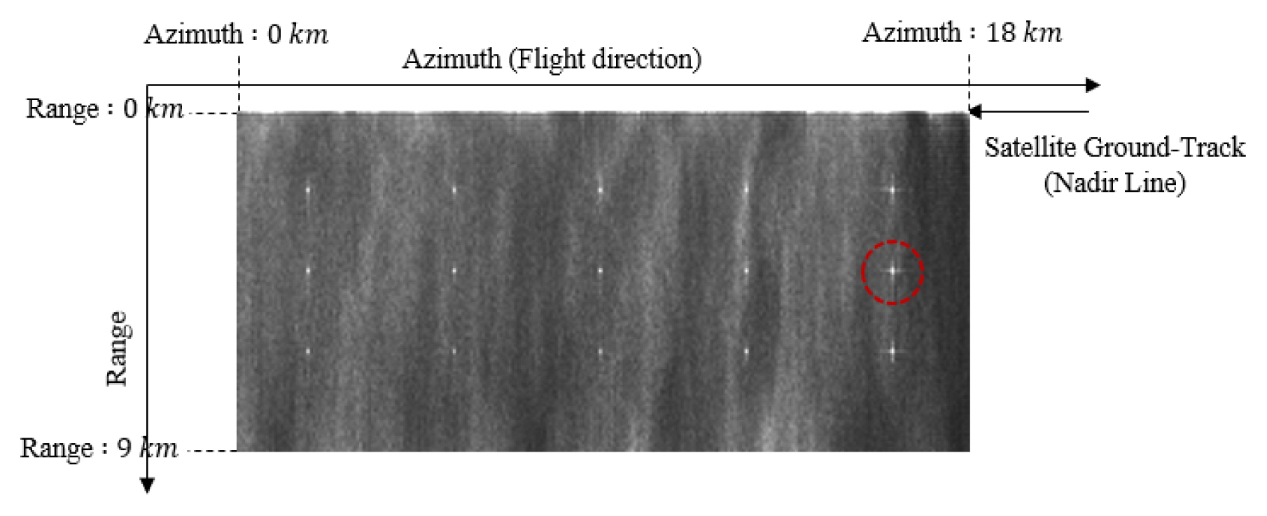
Since BRI is a fairly long value of 11.7 ms, the reflected beams in the beam-stacked data are uncorrelated in terms of phase, meaning that each observation was a completely independent look. Therefore, by simply accumulating the statistically independent beams in the stack, an accurate complex reflectivity function for the sample stripe cell can be obtained. This simple incoherent summation process that suppresses speckle and thermal noise is a multi-look process. By combining the multi-look processed data for all the sample stripe cells in the along-track direction, the two-dimensional image of the Sea of Okhotsk is obtained, as in Fig 14(a). The range resolution is about 70 m, and the azimuth resolution is about 77 m. This level of resolution is utilized when exploring certain natural features such as mountains, oceans, and forests [8].
8. Antenna Pattern Calibration
The bright line at the top of Fig. 14(a) is a nadir line that corresponds to the ground track of the satellite. The further away from the nadir line, the harder the image identification becomes. This is because the signal at other points is suppressed during the power normalization process because the nadir echo power is relatively strong compared to other points. Another critical factor causing this phenomenon is the antenna gain pattern [9]. Since the antenna gain in the cross-track decrease as the beam angle from the center beam becomes wider, the power of the reflected echo decreases. This is especially true for satellites, which have a long distance between the target surface and the radar platform. Therefore, a proper antenna pattern calibration process should be applied to show up the invisible sight. Fig. 14(b) shows the image with antenna pattern calibration applied. The full range of the image is clearly visible.
As mentioned earlier, since CryoSat-2 does not record the phase history of samples in the azimuth direction, the azimuth compression process is not required in the proposed ocean image formation algorithm. Therefore, the proposed SAR algorithm is less complex than other SAR algorithms.
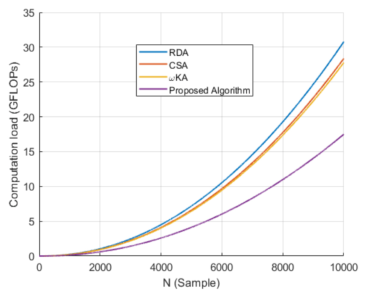
To quantitatively prove the low complexity of the proposed algorithm, a comparison of computational load with other SAR algorithms is conducted. The range Doppler algorithm (RDA), the chirp scaling algorithm (CSA), and the omega-K algorithm (ωKA) are selected for comparison because they are well known as efficient and accurate SAR algorithms [3]. Each SAR algorithm consists of some or all of the following three basic operations: fast Fourier transform (FFT/IFFT), phase multiplication, and interpolation. Since most of the computation quantity is in the above three operations, the computation quantity in other operations is neglected in the following analysis. Required floating point operations per second (FLOPs) for the three basic operations are given as:
N is the FFT length and M is the interpolation kernel length. Eq. (2) means the number of FLOPs required for the FFT of one-dimensional array of length N. Eq. (3) and (4) mean the number of FLOPs required per output point for each operation. Table 2 shows the number of basic operations constituting each SAR algorithm and their total computation load. For ease of comparison, it is assumed that the number of range lines and the number of azimuth lines of virtual raw data are the same as N. Fig. 15 visualizes the computational load of each SAR algorithm according to N. It can be seen that the proposed algorithm has the lowest computaional load.
Table 3 summarizes the advantages of the proposed algorithm compared to the SAR altimeter and image SAR algorithms. The proposed algorithm can utilize the Ku-band frequency even in the case of satellite platforms and is compatible with the altimeter system to extract images. As represented in Table 2 and Fig. 15, the computational load is also the lowest. Although the swath width of CryoSat-2 is somewhat narrower than the standard mode of other X-band image SAR satellites [10–12], it still has a wide enough swath width for SAR imaging.
IV. Validation of Algorithm
Since CryoSat-2 only searches areas with an almost uniform ground reflectivity, such as an ice glacier or open ocean, it is difficult to find any specific features in the image. Thus, one may hesitate to conclude that the proposed ocean image formation algorithm is reliable. Therefore, Section IV is added to prove that the algorithm is reliable; that is, Fig. 14 is a proper ocean image. As the SAR system is a linear system, the characteristics of the system can be analyzed through the impulse response. The impulse response of the SAR system refers to the system response to a single isolated scatterer, and such a scatterer is called a point target. The reflected signal from the point target is received through the SAR system and SAR processed. The processed signal in the SAR image is called the impulse response function (IRF). Essential SAR quality parameters, such as impulse response width (IRW) and peak side lobe ratio (PSLR), are estimated from IRF. Therefore, IRF has been obtained and analyzed to verify SAR performance in many studies [3, 13–16]. If the IRF of the proposed algorithm is similar to that of the existing SAR algorithm, so that appropriate values of the SAR quality parameters are obtained, the proposed algorithm can be said to be a reliable SAR algorithm. Therefore, a virtual point target simulation is conducted to validate the proposed algorithm.
ESA provided simulation results for the expected received signal for a single burst in the two-dimensional frequency domain. The simulation assumed that the radar altimeter is observing point targets and an ocean-like surface, respectively. The results are given in Fig. 16 [17]. This simulation result is reliable because the simulated result for an ocean-like surface and the actual received signal for an ocean-like surface are similar, as shown in Fig. 17. Expected received signals for a point target are assumed on the basis of these simulation results.
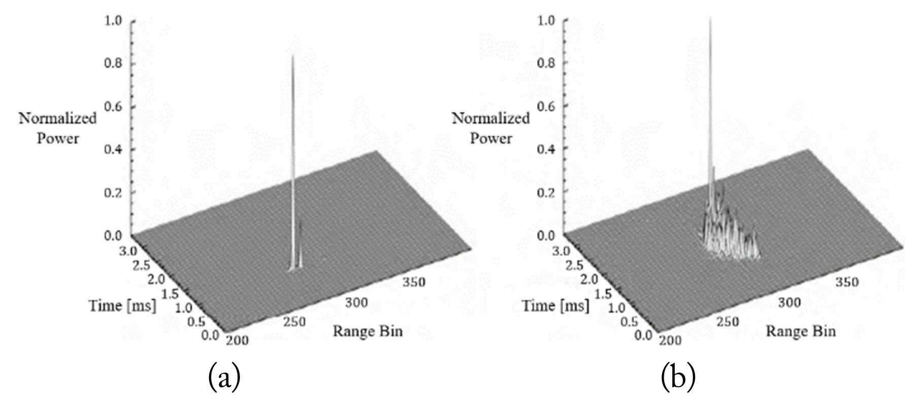
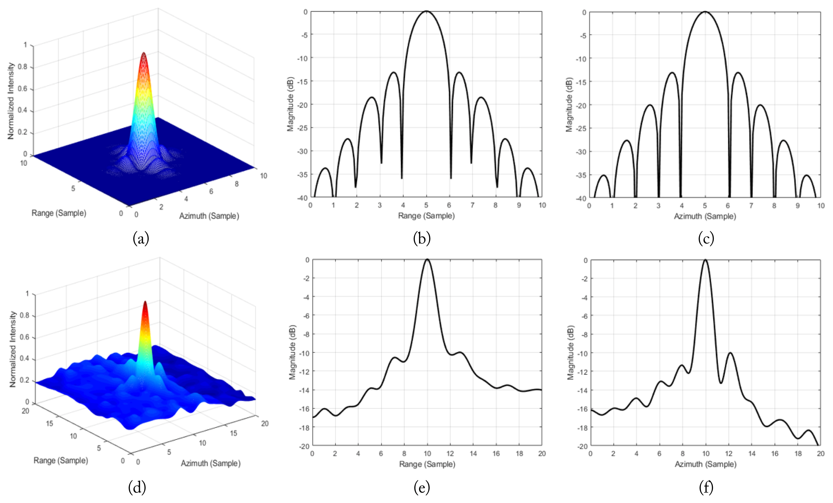
First, to analyze the performance of the proposed algorithm in an ideal case, we conducted a simulation assuming that only a point target exists. The expected received signals from a point target were used. These reflected signals became like Fig. 16(a) when two-dimensional Fourier transform was applied. The point target result of the proposed algorithm is given in Fig. 18(a)–(c). For visual clarity, interpolation by a factor of 16 was implemented. Fig. 18(a) shows the normalized intensity of IRF in 3D, and Fig. 18(b) and 18(c) show the one-dimensional profile of the IRF in the range and azimuth directions, respectively. IRW is about 1.1 samples in both directions and PSLR is about −13 dB in both directions. Considering that the general SAR algorithm produces a value of 1.0–1.5 for IRW and −13 dB for PSLR [3], the IRF of the proposed SAR algorithm satisfies the standards of the SAR algorithm.
Second, to analyze the performance of the proposed algorithm in a practical case, we conducted a simulation assuming that some point targets with high reflectivity, such as corner reflectors (point targets), are located over the ocean. The expected received signals from the point targets are added to the raw data of CryoSat-2. After that, by following the ocean image formation algorithm again for the modified CryoSat-2 data, we checked whether the point targets properly emerged over the ocean image. As shown in Fig. 19, virtual point targets are well emerged on the two-dimensional ocean image. The IRF of the circled point target in Fig. 19 is shown in Fig. 18(d)–18(f). Fig. 18(d) shows the normalized intensity of IRF in 3D, and Fig. 18(e) and 18(f) show the one-dimensional profile of the IRF in range and azimuth directions, respectively. The SAR quality parameter values of the proposed algorithm are given in Table 4 in both cases (ideal, practical). From the fact that the shape of the IRF is very similar to that of the existing SAR algorithm and the fact that SAR quality parameter values correspond to the general SAR algorithm, the reliability of the proposed algorithm is proved.
An ambiguity analysis is also performed to present another quantitative result that proves the reliability of the proposed algorithm. The analysis was performed for the range component and the azimuth component separately. The existence of azimuth ambiguities is caused by the antenna side lobes in the azimuth direction. Considering the antenna side lobe ambiguity effect in Section III-1, the azimuth ambiguity to signal ratio (AASR) can be obtained by the following equation [18]:
Sside is the signal power from side lobes of antenna, Smain is the signal power from main lobe of antenna, and Stotal is the total signal power from azimuth antenna beam pattern. Before the azimuth windowing, the AASR is about −13 dB and after the azimuth windowing, it is about −29 dB. Considering that the AASR of the typical SAR antenna is about −20 dB [18], it seems to be a reasonable value. On the other hand, the range ambiguity is significant for a typical space-borne SAR system. This is because the reflected signal of a specific pulse is received after several pulses have been transmitted. However, CryoSat-2 is free from range ambiguity problems since it utilizes burst mode pulse transmission with a long value of BRI (11.7 ms).
By conducting point target simulations (qualitative and quantitative results) and ambiguity analysis (quantitative results), we proved the reliability of the proposed algorithm.
V. Conclusion
A critical goal of this study is overcoming the frequency limits of the current SAR imaging satellites. SAR imaging satellites beyond X-band are difficult to design because of the limits of the Doppler frequency band that the system PRF can cover. In this paper, the author proposed a method to form SAR images using satellite (CryoSat-2) altimeter data. The operating frequency of CryoSat-2 is 13.575 GHz (Ku-band), which is beyond the current satellite SAR frequency limit (X-band). IRF and ambiguity analysis are conducted to provide quantitative results to show the applicability of the proposed algorithm. This paper also shows the possibility of two functions (SAR altimeter and image SAR) being implemented with only one radar. Due to unwanted tilting of the antenna, it was possible to obtain ocean images from SAR altimeter data. This means that, with a little intentional tilt, a satellite can switch its function from altimeter to image radar and vice versa. In addition, the research results are creative in that image reconstruction is implemented by non-image sensors. This research is a good example of how signal processing is key to a wide range of applications, from acquisition (altimeter data) to display (ocean image).