Through-the-wall radar imaging (TWRI) systems are an emerging technology that enables the detection of stationary or moving objects behind a wall from a position at a certain distance from the wall. TWRI systems use microwaves, which can easily propagate through walls to detect objects inside a building. They find various applications in many fields, such as the military, surveillance, indoor security, and search-and-rescue operations [1]. One of the several challenges is reducing the clutter present in the images produced by these systems to enhance their quality. Methods for reducing clutter in through-the-wall images include background subtraction, spatial filtering, image fusion, subspace projection, differential synthetic aperture radar (SAR), and entropy-based time gating [2–13]. These techniques have limitations. Background subtraction requires a scene with no targets, which is impossible in real-time scenarios [7]. Spatial filtering works only for homogeneous walls at low operating frequencies. Image fusion requires multiple through-the-wall radar images of the same scene generated from distinct locations, which is impossible for moving targets [7]. Subspace projection methods, such as singular value decomposition (SVD), principal component analysis, factor analysis, and independent component analysis, have the disadvantage that the total number of targets must be known a priori [7].

Moreover, these techniques can detect only single targets or multiple targets with the similar dielectric constant in the same scene [14]. However, in real-time scenarios, targets may not have similar dielectric constants. Thus, it is necessary to develop a technique for detecting contrast targets—that is, targets with different dielectric constants behind a wall in the same scene.

Few studies have explored methods for detecting targets with different dielectric constants. Recently, low-rank approximation (LRA) was developed to attenuate random noise in the received signal [14]. This paper proposes a novel technique that combines time gating and Gaussian mixture model–based LRA for contrast target detection—that is, the detection of targets with low and high dielectric constants behind a wall in the same scene. The proposed method works well with heavily cluttered through-the-wall images and enhances their quality.

The rest of this paper is structured as follows. Chapter II describes the through-the-wall imaging system model. Chapter III presents the proposed method for contrast target detection. Chapter IV reports and discusses the experimental results. Chapter V presents the conclusions.

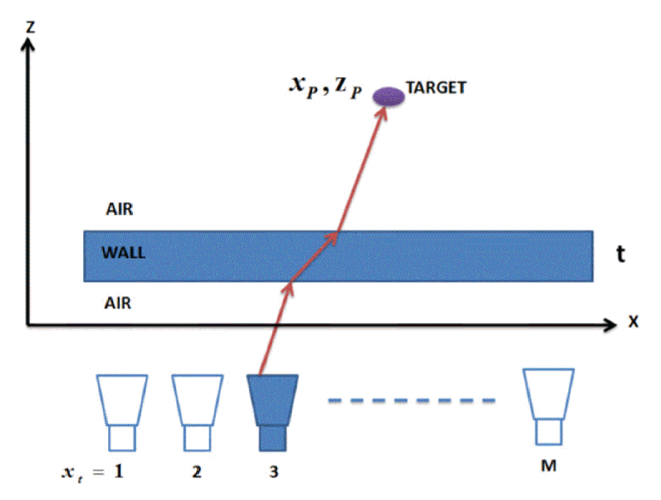
The imaging setup shown in Fig. 1 is placed at a certain distance from the wall, and data are acquired at M scan points along a horizontal direction parallel to the wall. The scan points represent the positions of the antenna of the stepped frequency continuous wave (SFCW) radar. The scene being imaged is situated behind the wall along the positive z-axis. At each scan point, the SFCW radar transmits and receives the signal scattered from the target. It transmits a wideband signal in step frequency mode, in which it sweeps through the allocated signal bandwidth via a series of narrowband signals of uniformly spaced center frequencies. The SFCW radar measures and records the magnitude and phase of the received signal scattered from the target for various frequencies at each spatial point. The scene is divided into pixels downrange and cross-range, represented by the z and x coordinates, respectively. The magnitude and phase of the scattered field from a P-point target located in position x_pi,_,z_pi behind the wall for various frequencies at different scan points are calculated as

where f_k is the frequency point, τ_pi is the propagation delay between the radar at m^th scan point and the pixel position, and a(x_pi,_,z_pi) is the target.

For each pixel, the corresponding propagation delay is calculated as [15]

where c is the speed of signal propagation in the air, v is the speed of the signal propagating through the wall, and l_airtowall, l_wall, and l_walltoair represent the signal’s distance from the radar when in front of the wall, inside the wall, and behind the wall at m^th scan point to the pixel at location x_pi,_,z_pi. The details of expression l_airtowall, l_wall, and l_walltoair are provided by Ahmad et al. [15].

After applying delays to the signal received in the frequency domain at each radar location to synchronize the signals arriving at each radar location and then summing the delayed signals, the value of a pixel at location x_pi,_,z_pi is calculated as [6]

Similarly, for the P-point scatterer in positions x_pi,_,z_pi, the value of each pixel at different P positions x_pi,_,z_pi is calculated as [6]

The proposed method for contrast target detection consists of three stages. In the first stage, clutter due to strong wall reflections is reduced using time gating based on the wall propagation time. In the second stage, delay-and-sum beamforming are applied to time-gated frequency domain data to obtain a focused image of the target. In the third stage, a Guassian mixture for LRA is introduced to detect targets with low dielectric constants and suppress noise.

Frequency domain data collected along M horizontal scan points are inverse Fourier transformed to obtain time domain data. The time domain data at m^th observation position can be written as [5]

where t ranges from 0 to (N–1) = signal bandwidth (BW) at Δt step intervals of 1/BW.

Upon discretizing time, S denotes the M X N matrix of the time domain data at M horizontal scan points, S = [S (m, n)], m = 1, 2, …, M–1, and n = 1, 2, …, N. M and N are the numbers of antenna positions and time samples, respectively.

To reduce wall clutter, the time domain data S (m, n) are time-gated based on the wall propagation time (W). The threshold is set to

where W is given by W=(d√ε + z_off), n is the time sample, z_off is the standoff distance, and c is the speed of light. The time trace after incorporating the threshold is calculated as

To compute the wall propagation time, the wall’s dielectric constant and thickness must be known a priori to compensate for the wall’s effects. The effective dielectric constant and thickness were estimated by exploiting the first two dominant echoes originating from the front and rear sides of a real building wall. Such walls are generally made of bricks and covered in a fine layer of plaster. Since the size of the inhomogeneities is smaller than the range resolution, the wall can be modeled as a homogeneous layer characterized by effective permittivity [16].

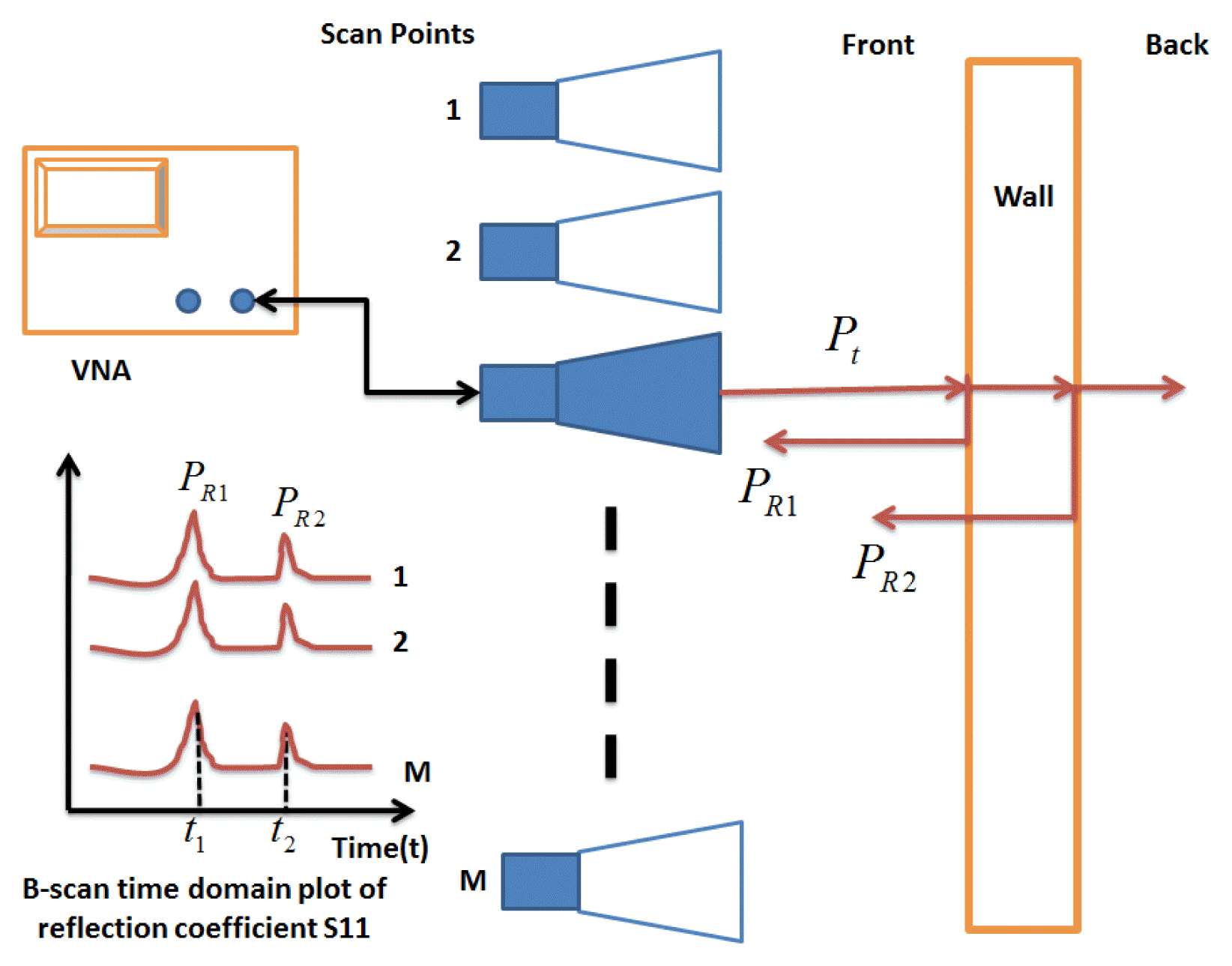
The signal transmitted from the antenna at a certain scan point has power P_t. The signal propagates toward the wall and is incident on the front side of the wall, as shown in Fig. 2. A signal with a certain portion of power is reflected, and a signal with a certain portion of power propagates through the wall.

The received signal reflected from the front side of the wall has power P_R1 and appears as a peak at time point t₁. The received signal reflected from the rear side of the wall has power P_R2 and appears as a peak at time point t₂. P_R1 can be written as [17, 18]

where P_L1 is the total loss, which includes the cable loss as the signal propagates from vector network analyzer VNA to the antenna and the path loss between the antenna and the front side of the wall, and |Γ| is the magnitude of the reflection coefficient at the interface of the front side. P_R2 can be calculated as [17, 18]

where P_L2 is the total loss, which includes the cable loss as the signal propagates from VNA to the antenna and the path loss between the antenna and the rear side of the wall, and |Γ| is the magnitude of the reflection coefficient at the interface of the rear side.

Considering the cable and path losses to be the same, a mathematical relation between P_R1, P_R2, and the reflection coefficient can be written as

Where |Γ| represents the reflection coefficients at the interfaces of the front and rear surfaces of the wall, α is the wall attenuation constant, and d is the wall thickness, which is given by

where σ is the electrical conductivity of the wall, η is 377 Ω, and c is the speed of light in free space.

Substituting Eqs. (11), (12), and (13) for (10), we can express Eq. (10) in terms of other variables as follows:

The wall’s dielectric constant and thickness can be obtained by exploiting P_R1 at time point t₁, P_R2 at time point t₂ from time domain plot, and time delay Δτ=t₂-t₁. Thus, the dielectric constant and electrical conductivity of the wall can be estimated by formulating a proper fitness function and minimizing it using an efficient searching technique, a genetic algorithm, which can be written as

Once the wall’s dielectric constant has been obtained, its thickness d can be computed using Eq. (13). To obtain P_R1 and P_R2 at time points t₁ and t₂ at all scan points, first, S(m, n) are added up in the time domain.

Next, the maximum value of Sum(n) is obtained, and the threshold is set as

where α < 1 is the tolerance band. Then, based on Eq. (17), the peak P_R1 and P_R2 values and corresponding time points t₁ and t₂ can be obtained for all M scan points as follows:

After the time gating process, the time domain data S_T(m, n) are Fourier-transformed and further processed by applying delay-and-sum beamforming using Eq. (4) to produce a focused image of the target. Although the echo of high dielectric constant target is strong, the echo of targets with low dielectric constants is comparable to noise. Therefore, LRA is introduced to reduce noise based on the Gaussian mixture model to detect a target with a low dielectric constant along with a target with a high dielectric constant. After applying SVD, the beamformed image matrix I can be expressed as [14]

where U and V are M X M and N X N unitary matrices, S = diag(λ₁, λ₂, ..., λ _r), and λ is a singular value in the order of λ₁ > λ₂ >………. λ_r > 0. U and V are eigen vectors of I.

It was observed that the boundaries of the singular values corresponding to the target and noise were not clearly defined. Hence, it is not feasible to exploit singular values accurately corresponding to the target. Thus, a Gaussian mixture model is used to segregate the singular values corresponding to the target and noise.

After normalizing λ(r), the singular values are modeled as a mixture of Gaussian distributions. The Gaussian components in the mixture are composed of target and noise components, and the overlapping boundaries of the singular values corresponding to the target and noise are separated using clustering based on maximum a posteriori. The singular values are modeled using an expectation–maximization algorithm to obtain the parameters of the Gaussian mixture, which is given by [19]

Where μ_K is the mean of the k-th Gaussian component, σ_K² is the variance of the k-th Gaussian component, K is the number of Gaussian components, K = 1 represents the target component, K = 2 represents the noise component, and G(r) is the Gaussian component given by

To segment the singular values corresponding to the target from those corresponding to noise, clustering that assigns each data point to one of the two mixture components in the Gaussian mixture model based on posterior probability is performed as

The center of each cluster is the mean of the corresponding mixture component. After obtaining n singular values corresponding to the target from matrix S and setting other values to zero such that S̄ =S (1 : n, 1 : n), the LRA matrix is computed as

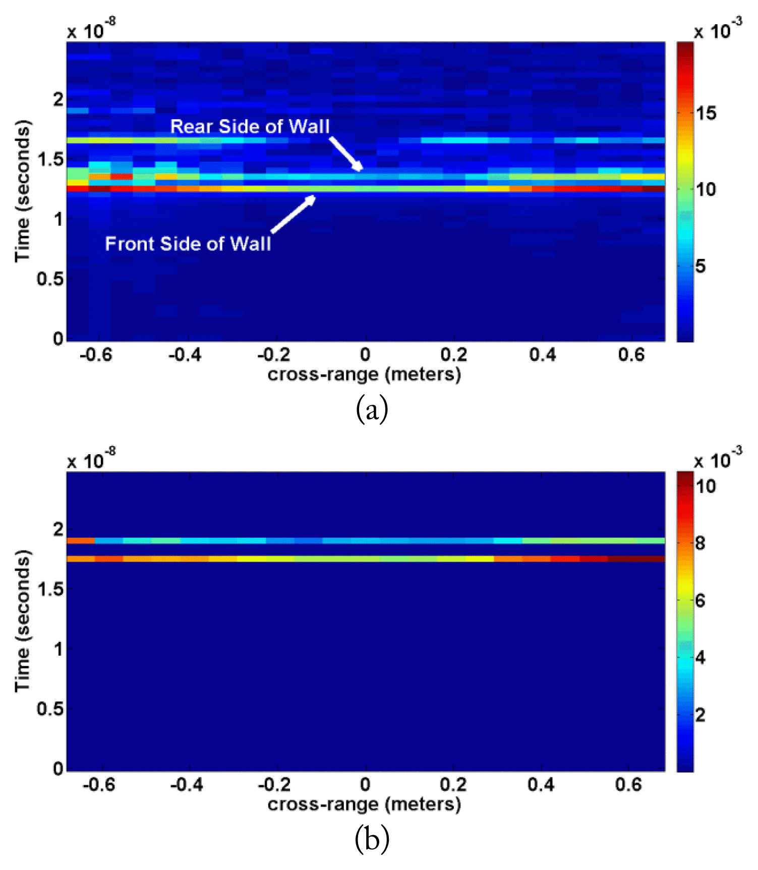
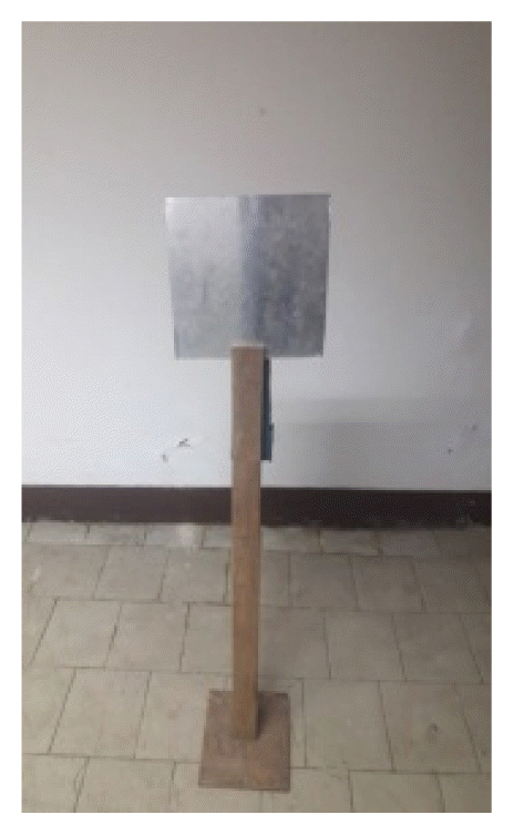
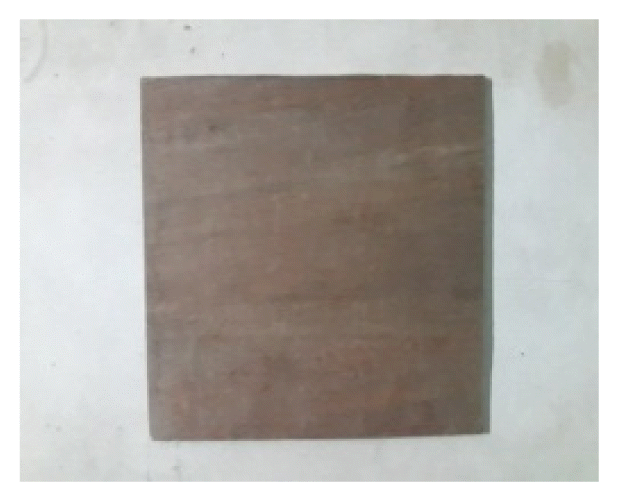
To evaluate the image enhancement capability of the proposed method, four TWRI scene was simulated using two targets, one with a low dielectric constant (wood) and one with a high dielectric constant (metal), behind a wall (Table 1). Photographs of the targets and their measured radar cross-section values are shown in Table 2. An experiment was performed using SFCW radar. Scattering parameter S₁₁ was measured for 201 frequency points in the frequency range of 3.5–5.5 GHz at 27 scan points along the horizontal direction. The imaging setup was placed at a distance of 2.2 m from the front side of the wall. Fig. 3(a) shows the raw B-scan image. Fig. 3(b) shows the image of the B-scan obtained using Eq. (18) to extract the peak P_R1 and P_R2 values from the front and rear sides of the wall at time points t₁ and t₂, respectively. The wall’s thickness and effective permittivity after incorporating the peak P_R1 and P_R2 values and time delay τ were computed using Eqs. (13) and (15).

The wall’s thickness and dielectric constant were found to be 14.4 cm and 6.4, respectively. To validate the results, the wall’s effective permittivity was computed using a wall insertion transfer function in a manner similar to that described by Chandra et al. [20]. The wall’s effective permittivity obtained was 6.5 and actual thickness of wall was 14.5cm. The wall’s effective permittivity estimated using the frequency domain method was in good agreement with that obtained using the method proposed by Chandra et al. [20].

After estimating the wall parameters, the frequency domain data were processed to enhance the image using the proposed method. The image was then assessed in terms of target-to-clutter ratio (TCR), calculated as [6]

where A_t is the target area, A_c is the clutter area, N_t is the number of pixels in the target area, and N_c is the number of pixels in the clutter area.

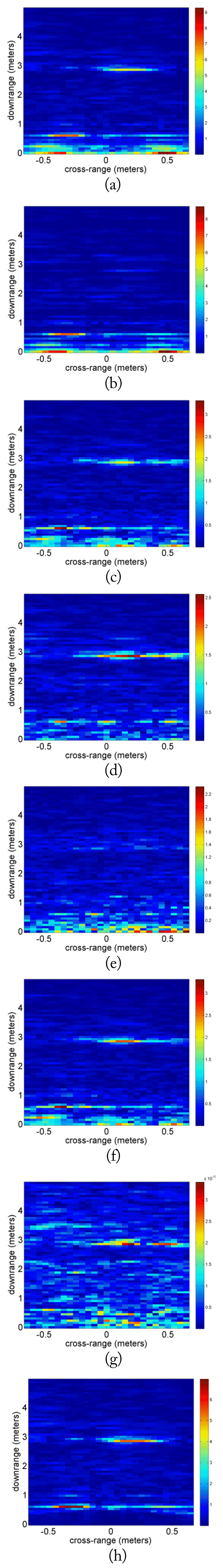
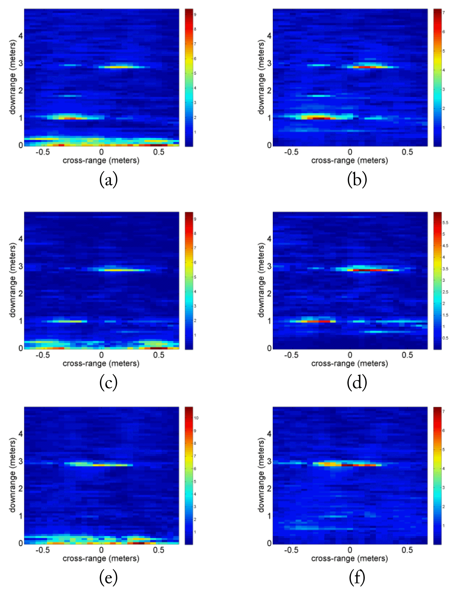
Fig. 4 shows the through-the-wall radar image of the scene behind the wall after applying a delay-and-sum beamforming algorithm directly to the frequency domain data—that is, scattering parameter S11 without clutter reduction and with clutter reduction using different techniques. The proposed method produced an enhanced image and was capable of detecting the target with the low dielectric constant (wood) along with the target with the high dielectric constant (metal) in the same scene.

Table 3 presents a comparison of the proposed method with other clutter reduction techniques in terms of TCR for the images shown in Fig. 4. The proposed method obtained the highest TCR (130.1).

Fig. 5 shows through-the-wall radar images with delay-and-sum beamforming applied using the proposed method for Scenes 2, 3, and 4. The proposed method enhanced the quality of the images, demonstrating its effectiveness with different target types and arrangements.

To determine the margin of error needed for this technique to work, the TCR of the Scene 1 image obtained using the proposed method was calculated with varying wall dielectric constant and thickness values by 5%. The obtained TCR values are shown in Table 4 and 5. The TCR decreased as the dielectric constant changed by 20% and as the thickness changed by 10%. Thus, an estimation accuracy of more than 20% for the dielectric constant and more than 10% for thickness is sufficient for this method to work.

This study proposes a novel method for contrast target detection. The inherent problem of strong clutter due to the wall and its residual due to the interactions between the wall is addressed using time gating based on the wall propagation time, and noise is reduced using LRA based on a Gaussian mixture model.

The proposed method was validated using through-the-wall images generated using SFCW radar. The experimental results showed that this method can detect targets with a low dielectric constant in the presence of targets with a high dielectric constant in heavily cluttered through-the-wall images of the same scene with satisfactory accuracy.

The proposed technique was also compared to existing clutter reduction techniques, such as entropy-based time gating, SVD, average trace subtraction, differential SAR approach, robust PCA, and entropy-based low-rank approximation. The proposed method showed highest TCR (130.1).

An estimation accuracy of more than 20% for the wall’s dielectric constant and more than 10% for its thickness is sufficient for the proposed method to work. This method is quite effective in reducing clutter due to inhomogeneous walls, provided that inhomogeneity is smaller than the range resolution.