Design and Fabrication of a Compact 2D Phase Comparison Direction Finder
Article information
Abstract
In this study, a compact, low-power 2D phase comparison direction finder was designed and fabricated. For the design of the direction-finding (DF) receiver, a 2D phase comparison DF equation was derived from the structure of four uniformly arranged antennas, and the main design parameters were derived from the receiver’s system parameters. Based on the derived DF equations and design parameters, a DF receiver was designed, and a direction finder was fabricated. A comparison of the fabricated direction finder to a simulation model showed that its performance was comparable to the simulated performance and satisfied the system parameters. Moreover, a comparison of the theoretical, simulated, and actual injection and radiation DF precision showed that the fabricated direction finder had performance consistent with that indicated by the theoretical and simulation results and DF precision within 0.5°.
I. Introduction
Direction-finding (DF) technology is based on active and passive DF methods. The active method detects a target’s direction by transmitting signals, such as radar, and receiving the signals reflected by the target. The passive method detects a target’s direction by receiving a signal from a signal source. The passive method has the advantage of being undetectable by alarm systems (such as radar warning receivers and electronic support equipment) because it does not transmit radio waves. Moreover, it requires less power than the active DF method, and its hardware can be relatively small. On the other hand, it has the disadvantage of being unable to detect a target if the signal transmission of the source is stopped [1, 2].
The passive DF method is divided into amplitude comparison, phase comparison, and mono-pulse DF. The phase comparison DF method employs the angle of arrival (AOA) technique using the phase difference of the signals received by two or more antennas arranged on one baseline. This technique is widely used to enable DF in a short period and provides good accuracy [1–3].
Conventional phase comparison DF studies have mainly investigated 1D DF, which detects only the azimuth angle [4–7]. Conventional DF receivers are typically heterodyne [1, 4, 8–11], using a local oscillator and analog mixer to shift the signal band to theintermediate frequency (IF). The Nyquist sampling theorem is then used, the sampling of which is more than twice the maximum frequency.
However, heterodyne receivers are limited by their great size, weight, and power (SWaP) [12, 13]. Recent 2D DF can detect both the azimuth and elevation angles but requires SWaP reduction due to limitations in platform size [2, 3, 7]. Several studies on small direction finders have been conducted [7–9]. However, most small direction finders are 1D and use the multiple signal classification (MUSIC) algorithm. These direction finders have excellent performance, but they rely mostly on post-processing and therefore have poor real-time performance. To simplify the structure while maintaining performance, it is necessary to develop a direct radio frequency (RF)-sampling DF receiver. To that end, in this study, a 2D phase comparison DF receiver using direct RF sampling was designed and fabricated to reduce SWaP. The performance of the fabricated DF receiver was compared to the performance of the RF-receiving part obtained from a simulation model.
II. 2D Phase Comparison df Equations
The 2D phase comparison DF equation was derived from a structure of four uniformly arranged antennas, and the main design parameters of the direct RF sampling–based receiver were derived according to the system parameters.
1. 2D Phase Comparison DF Model
The structure of the 2D phase comparison DF, which estimates the relative azimuth and elevation of the received signal, is shown in Fig. 1. The structure is simple, consisting of four uniformly arranged antennas to achieve a compact size and to obtain the azimuth and elevation baselines.

Uniform array antenna using four elements.
The incident signal source is the ⇉ vector of the spherical coordinate system. When the ⇉ vector is expressed by the rectangular coordinate system, the relative phase difference (between the elevation (φ12) and the azimuth (φ34) angles can be calculated using Eqs. (1) and (2), respectively [2, 5]:
where β is the phase constant (radians per meter), ⇉ is the unit vector for the direction of incidence of the signal source, d⃗ij is the baseline length between antennas i and j (in meters), and xi, yi, zi is the position of antenna i. To solve Eqs. (1) and (2), the known position of the antenna is used in Eqs. (3) and (4):
From Eqs. (3) and (4), the azimuth and elevation angles can be calculated using Eqs. (5) and (6):
In Eq. (6), the elevation angle is required to estimate the azimuth angle. Therefore, elevation is independent of the azimuth, but the azimuth depends on elevation.
DF precision can be interpreted as a change in the azimuth and elevation angles [2] and can be calculated by modifying Eqs. (5) and (6), respectively, as follows:
where, dθAZ and dθij are the changes in the azimuth and elevation angles, respectively, dφij is a change in the phase difference between antennas i and j, and SNRi is the signal-to-noise ratio (SNR) of the receiving channel connected to antenna i. In Eqs. (7) and (8), DF precision depends on the SNR, baseline length, and azimuth and elevation angles.
2. DF Receiver Design
In the direct RF sampling receiver, the received signal is amplified in the desired bandwidth through a band-pass filter and amplifiers in the RF-receiving part and then sampled in an analog-to-digital converter (ADC) without IF conversion [13, 14]. Processing after sampling is performed by digital processing parts, such as the field-programmable gate array (FPGA) and the digital signal processor. Table 1 shows the system parameters of the DF receiver design.

System parameters
The SNR for satisfying AOA precision can be estimated by the inverse calculation of Eqs. (7) and (8). A simulation was performed considering the noise effect using the MATLAB. The maximum simulation result was 23.8 dB. Considering the design margin, the SNR was set to 25 dB.
The thermal noise based on the receive bandwidth is calculated as −96.22dBm from Eq. (9) [15, 16]:
where NT and BW represent the thermal noise based on the received bandwidth and bandwidth, respectively. As a result of Eq. (9), thermal noise is greater than the receiving sensitivity signal. Therefore, gain improvement using the fast Fourier transform (FFT) is needed. The FFT number for satisfying the minimum detectable SNR can be calculated using Eq. (10) [15]:
where Pmin is the receiver’s sensitivity, NF is the noise figure, and M is the FFT number. Considering the design margin, the noise figure is assumed to be 5 dB. The minimum FFT number (M) calculated using Eq. (10) was 4096.
When sampling a continuous signal in the time domain, the spectrum of the signal is repeated at each sampling frequency, which is called an alias [12, 13, 17]. Direct RF sampling is a method of sampling a passband signal by setting a sampling frequency so that the spectra do not overlap. To avoid overlapping aliases, the sampling frequency (fs) must satisfy the following condition [13]:
where fL and fH represent the minimum and maximum frequencies of the signal, respectively, B is the signal bandwidth, B=fH–fL, ⌊ x ⌋ is the maximum integer that is not greater than x, and k is the number of repeating spectra between the signal band and the baseband.
To reduce aliasing noise repeated outside the signal band during direct RF sampling, the band-pass filter removes it before sampling so that the noise spectrum does not overlap with the signal spectrum. The distance between the repeating spectra is increased so that the noise spectrum does not overlap with the spectrum of the signal band. Therefore, increasing the sampling frequency can increase the bandwidth of the band-pass filter and reduce the aliasing noise even if the skirt characteristic of the filter in the transient region is not sharp [12].
The ADC of the direct RF sampling receiver of the 2D phase comparison direction finder is an AD9684 (Analog Devices) with 14-bit resolution and differential signal output to reduce noise effects [18]. It has a sampling frequency of up to 500 MSPS to satisfy the bandwidth of the system parameters and is composed of a two-channel ADC to satisfy the compact size requirement.
III. Simulation of the 2D Direction Finder
A simulation-based 2D DF receiver was designed using a virtual system simulator (VSS) and Simulink based on the derived design parameters and equations, and its performance was verified.
1. 2D Direction Finder Simulation Model
A system diagram of the 2D direction finder design is shown in Fig. 2. The array antenna part is composed of four patch antennas satisfying the bandwidth of 60 MHz at the center frequency for RF signal reception. The RF-receiving part amplifies and filters the received signal, outputs it to the input part of the ADC, and generates an in-phase/quadrature signal through direct RF sampling in the ADC. Digital signal processing is then performed by the FPGA and microcontroller unit/central processing unit.
Configuration diagram of the direction finder.
In the simulation model, the RF-receiving part was implemented using the VSS, and the digital signal–processing part after the ADC was implemented using Simulink. Fig. 3 presents a detailed schematic diagram of the RF-receiving part. The RF-receiving part receives a signal from −10 to −100 dBm and passes an output of 3 to −57 dBm to the ADC of the signal-processing part to satisfy the input dynamic range and instantaneous dynamic range. As the input signal strength range is 30 dB greater than the output signal strength range, the RF-receiving part performs an automatic gain control (AGC) of 30 dB to fit it into the ADC dynamic range of the signal-processing part. In the AGC flow, the RF signal received from the antenna through a directional coupler and an RF detector is converted to a voltage signal and then entered into the FPGA of the signal-processing part through a comparator composed of an op-amp, which outputs a high or low signal. The FPGA controls the gain of the digital variable gain amplifier (DVGA) in the RF-receiving part according to the local signal from the input signal strength, thereby controlling the gain of the RF-receiving part. If the strength of the received RF signal is greater than −40 dBm, the comparator outputs a low signal so that the FPGA of the signal-processing part sets the DVGA gain to 10 dB and the path gain of the RF-receiving part to 13 dB. If the strength of the RF signal is less than −40 dBm, the comparator outputs a high signal so that the FPGA of the signal-processing part sets the DVGA gain to 40 dB and the path gain of the RF-receiving part to 43 dB. This process implements an AGC of 30 dB, allowing the RF-receiving part to output a signal within the dynamic range of the ADC.
Configuration diagram of the RF-receiving part implemented using the VSS.
Fig. 4 shows the 2D phase comparison DF receiver designed using Simulink. The DF receiver consists of a signal source generator, a phase difference calculator, an AOA estimator, and an accuracy estimator.
Simulation diagram of the digital signal–processing part implemented with Simulink.
The signal source generator simulates four channels of input signals to the DF receiver, and the phase difference calculator calculates the phase difference of the input signal from the signal source generator based on the equations presented in Chapter II. The accuracy calculator calculates the relative azimuth and elevation angles based on the results of the phase difference calculator. To reduce the influence of noise and ensure accurate DF, the average of the azimuth and elevation AOA is outputted for every certain number of worst SNR signals during DF. The standard deviation of the DF result is outputted to calculate the DF precision.
2. Simulation Results
Figs. 5–7 present the simulation results of the RF-receiving part implemented using the VSS. Figs. 5–7 also show the test results of the received bandwidth, instantaneous dynamic range, and AGC of the simulation model, respectively. For the instantaneous dynamic range test, a simulated 60-MHz noise signal was injected, and simulated signals of –10 and –70 dBm were simultaneously injected into the center frequency and a frequency of 15 MHz away from the center frequency. For the AGC test, simulated signals of −50 and −30 dBm were injected.
Input bandwidth simulation results.
Instantaneous dynamic range simulation results.

AGC simulation results.
The simulation results showed that the designed digital receiver satisfied the received bandwidth of 60 MHz and the receiver sensitivity of −100 dBm. Moreover, the results showed that it was possible to obtain an instantaneous dynamic range of 62.198 dB and an AGC of 42.69 and 12.67 dB according to the input signal strength.
The theoretical DF precision calculated using Eqs. (7) and (8), and the DF precision of the simulated DF receiver are shown in Figs. 8 and 9. For the error model, the white Gaussian noise model, which has been widely used in measurement error models, was used [19, 20]. In calculating DF precision, the SNR applied the derived design parameter of 25 dB.

Theoretical DF precision. (a): azimuth, (a): elevation.
DF precision simulation results. (a): azimuth, (a): elevation
The results showed that the overall theoretical and simulated DF precision trends were similar. The azimuth precision was worse than the elevation precision. Both the azimuth precision and the elevation precision became worse toward the edge of the field of view. The elevation precision did not change when the azimuth angle changed but changed when the elevation angle changed. This confirmed the predictions of Eqs. (5) and (6), according to which elevation does not depend on the azimuth; thus, there is no change in DF precision according to azimuth changes. Conversely, because the azimuth depends on elevation, the azimuth precision is affected by elevation changes.
IV. Fabrication of the 2D Direction Finder
The 2D phase comparison direction finder was fabricated based on the simulation model. Channel and radiation correction methods were used to correct the difference between the inevitable theoretical and actual phase difference distributions. Measurement methods were used for the DF precision of injection and radiation, and the simulation and test results were compared.
1. Fabricated 2D Direction Finder
Fig. 10 shows the fabricated direction finder based on the configuration diagram (Fig. 2) and the simulation model. The direction finder consists of three parts, is 18 × 13 cm in size, and is stacked. Fig. 10 also shows the RF-receiving, ADC, and digital signal–processing parts.

The fabricated 2D direction finder. (a): RF-receiving part, (b): ADC part, (c): digital signal–processing part.
While fabricating the direction finder, a two-channel ADC was used for miniaturization, and a Zynq-XC7Z100 (Xilinx), which integrates an FPGA and a CPU, was employed [21].
Table 2 shows a comparison of the characteristics of the proposed direction finder to those of previously fabricated direction finders. The size of the proposed direction finder is smaller than those of Park and Kong [8] and Kang and Lee [9], which have a heterodyne structure. Although the proposed direction finder is larger than Kataria et al. [7], the latter is one-dimensional. Therefore, its size would inevitably increase if it were extended to two dimensions. Moreover, Kataria et al. [7] used the MUSIC technique for precise DF, which makes real-time DF difficult due to postprocessing. Conversely, the proposed direction finder is capable of real-time DF.
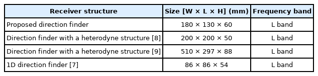
Size comparisons according to receiver structure
Miniaturized patch antennas with circular polarization (CP) are widely used in current wireless communication systems. CP antennas attenuate multipath effects and allow information transmission regardless of the receiver’s orientation with reference to the transmitter [22]. For this reason, CP was used in the antenna of the proposed direction finder. Fig. 11 shows the fabricated antenna’s configuration. Four patch antenna elements were arranged for the azimuth and elevation baselines perpendicular to each other and fabricated to satisfy the 60-MHz bandwidth at the center frequency. Table 3 shows the antenna’s main performance.

The antenna of the fabricated direction finder.
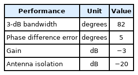
Performance of the direction finder’s antenna
2. Phase Difference Correction of the Direction Finder
When fabricating a phase comparison direction finder, practical errors in the manufacturing process and component characteristics can cause amplitude and phase mismatches between channels. Precise DF can be achieved by correcting such mismatches on the RF front end. This process is called channel correction. The compensation, including the antenna characteristics obtained from a radiation test, is called radiation correction. In this study, the performance of the direction finder was verified after channel correction and then after radiation correction, including the antenna.
In channel correction, the phase differences between the channels of an RF-receiving part are measured using a reference measurement device, and then an injection correction table is generated and inserted into the direction finder. In this study, the same four-channel output signals were equally generated using the reference measurement device and connected to the RF input ports of the DF receiver. The phase differences between the channels were then measured. The phase differences were those from the RF-receiving part, which precedes the ADC part. As shown in Fig. 12(a), the injection table was created according to the frequency (f), azimuth (AZ_–n ~ AZ_n), and elevation (EL_–m ~ EL_m) using the measured azimuth baseline phase difference (φAZn,m) and the elevation baseline phase difference (φELn,m) between channels 3 and 4. It was subsequently inserted into the direction finder, which then outputted the DF result by calculating the minimum distance between the measured phase difference and the phase difference in the table.
Direction-finding correction table: (a) injection and (b) radiation.
In radiation correction, a radiation correction table is generated using the phase differences of the signal measured by the direction finder according to the positioner’s rotation and is then inserted into the direction finder. A transmitted signal is radiated from a transmitting antenna after installing the direction finder on the positioner in an anechoic chamber. In this study, to minimize the multipath effects in the anechoic chamber during radiation correction, DF was performed by inserting the phase differences of the theta–phi axis according to the positioner’s rotation axis into the radiation correction table, as shown in Fig. 12(b), and then converting it to the angle of the AZ–EL axis [23]. The radiation correction table according to the frequency (f), theta (T_0 ~ T_n), and phi (P_0 ~ P_360) consisted of the phase difference value of the azimuth baseline (φTn,m) and the elevation baseline (φPn,m).
3. 2D Direction Finder Performance Analysis
To measure the performance of a fabricated direction finder, a reference instrument is needed. In this study, an E8257D signal generator and an N9020A spectrum analyzer (Agilent) were used as the reference generator and measurement device, respectively. Fig. 13(a) shows the test configuration diagram for measuring the dynamic range, and Fig. 13(b) presents the test configuration diagram for measuring the bandwidth, AGC, and receiver sensitivity.
Configuration diagram: (a) instantaneous dynamic range and (b) bandwidth, AGC, and receiver sensitivity.
To compare the test results with the simulation results, the same input signal conditions were used. To measure the receiver’s sensitivity, the minimum input power at the point where signal detection and DF were possible was measured by reducing the input signal power in 1-dB increments starting from −100 dBm. To measure the bandwidth, tone signals were injected simultaneously at both ends of the bandwidth and center frequency.
The test results indicated a receiver sensitivity of −102 dBm and bandwidth satisfying the system parameter. Fig. 14 shows the instantaneous dynamic range test results at input signal powers of −70 and −10 dBm. Fig. 15 presents the AGC test results at input signal powers of −30 and −50 dBm.
Dynamic range test results.
AGC test results. (a): −30 dBm, (b): −50 dBm.
The test results showed that the performance of the fabricated direction finder was consistent with that indicated by the simulation results. It was possible to ensure an instantaneous dynamic range of 62.7 dB and an AGC with a gain of 13.35 dB at an input signal power of −30 and 44.11 dB at an input signal power of −50 dBm.
To systematically analyze the performance of the direction finder, the injection DF precision of the DF receiver except the antenna and then the radiation DF precision of the direction finder including the antenna were measured. The injection DF precision measurement determined the DF precision of the DF receiver, which performed the channel correction. For this purpose, as shown in the test configuration in Fig. 16, the injection DF precision was measured using a reference signal generator. After generating the phase values of the four-channel output of the reference signal generator, which matched the azimuth and elevation to be measured, using Eqs. (3) and (4), the four-channel output ports were connected to the RF input port of the DF receiver. The DF results of the received signal were then transmitted to a personal computer through an RS-232 serial interface connected to the DF receiver. Table 4 shows the performance of the reference signal generator used in the test.
Injection DF precision test configuration.

Performance of the reference signal generator
The radiation DF precision measurement determined the DF precision of the direction finder while performing radiation correction in the anechoic chamber. Fig. 17 shows the test configuration used. The direction finder estimated the DF result according to the angle of the rotator’s theta–phi axis in the chamber, converted it to the angle of the AZ–EL axis, and then transmitted a serial message. Figs. 18 and 19 illustrate the injection DF precision of the fabricated DF receiver and the radiation DF precision of the direction finder. DF precision was measured at the same receiver sensitivity as the simulation conditions for comparison.
Radiation DF precision test setting with the theta–phi axis in the chamber.
Injection DF precision test results. (a): azimuth precision, (b): elevation precision.
Radiation DF precision test results. (a): azimuth precision, (b): elevation precision.
The test results showed that the performance of the fabricated direction finder was similar to that indicated by the simulation results. However, the injection and radiation DF precisions were 1.86 times worse than the simulated precision. During channel correction, phase measurement errors occur because of changes in the test configuration, such as RF cable tightening and temperature changes. Radiation correction includes the effects of channel correction errors and changes in the phase difference characteristic of the antenna. Changes in the phase difference characteristic of the antenna are caused by changes in the electrical length of the baseline due to an insufficient antenna ground plane and the dielectric constant and size errors during the fabrication of the antenna. The differences between the simulation and measurement results were due to such errors.
Table 5 shows the maximum values of the theoretical, simulated, injection, and radiation DF precision in the boresight. The DF precision was within 0.5° in the boresight.
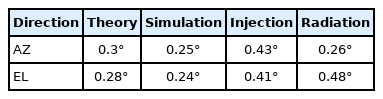
Maximum DF precision values in the boresight
Finally, the performance of the proposed direction finder was compared to that of a previously fabricated direction finder[7]. The results showed that, although the proposed direction finder is larger than the previously fabricated direction finder, it can provide excellent 2D DF in real time. The comparison results are shown in Table 6.

Comparison of the performance of the proposed direction finder with that of a previously fabricated direction finder
V. Conclusion
In this study, a 2D phase comparison direction finder was designed and fabricated to estimate the relative azimuth and elevation angles of a signal source. A direct RF sampling–based digital receiver was designed to reduce SWaP. For the design of the DF receiver, a 2D phase comparison DF equation was derived from the structure of four uniformly arranged antennas, and the main design parameters were derived from the receiver’s system parameters. Based on the derived DF equations and design parameters, a simulation-based DF receiver was designed, its performance was verified, and then a direction finder was fabricated. A size smaller that those of existing heterodyne-type direction finders was achieved. A phase difference correction method was used for its fabrication.
The performance of the fabricated DF receiver was compared with the simulation model. The results showed that the performance of the fabricated DF receiver was similar to that of the simulation model. The fabricated DF receiver had an instantaneous dynamic range of 62.7 dB and an AGC according to the input signal strength. The theoretical, simulated, injection, and radiation DF precisions were compared to analyze the DF performance of the fabricated direction finder. The results showed that the performance of the fabricated direction finder was consistent with that indicated by the theoretical and simulated results. Although its precision was 1.9 times worse than that predicted by the theoretical results because of phase measurement errors, it was within 0.5° precision in the boresight. Taken together, the results show that it is possible to fabricate a 2D phase comparison direction finder with excellent performance and reduced SWaP.
References
Biography

Jong-Hwa Jeon received an M.S. degree from the Department of Electronics, Radio Sciences, and Information Communications Engineering of Chungnam National University in 2018. He worked as a researcher at the Agency for Defense Development from 2018 to 2019. He is currently a researcher at the Jeonbuk Institute of Automotive Convergence Technology.

Myoung-Ho Chae received an M.S. degree from the Department of Radiowave Engineering of Chungnam National University in 2012. He is currently a senior researcher at the Agency for Defense Development.