Calculation of Normalized Site Attenuation for Calculable Dipole Antennas
Article information
Abstract
When a pair of calculable dipole antennas (CalDAs) with a 3-dB hybrid balun is used for a validation test of a constructed open area test site (OATS), the theoretical normalized site attenuation (NSA) curves of an ideal OATS for the CalDAs are required. This paper presents a method to calculate this theoretical NSA in the frequency range of 30 MHz to 1 GHz. The theoretical NSA was directly derived using the power mismatch and dissipative loss concepts of an NSA measurement system. Accurate antenna factors (AFs) above the ground plane were also needed and calculated to obtain the theoretical NSA. When free-space AFs are used to determine the measured NSA, AF correction factors known as mutual impedance correction factors are needed. Both free-space AFs and AF correction factors were also considered.
I. Introduction
An open area test site (OATS) is used to calibrate electromagnetic compatibility (EMC) antennas for field strength measurements and radiated emission measurements. The evaluation methods used to verify the performance of OATS use site attenuation (SA), which is known as classical site attenuation (CSA) [1–6], and of normalized site attenuation (NSA) [7]. The NSA concept is very useful because the subtraction of the AFs from CSA makes the NSA independent of the antenna type and has become the standard method for the validation of OATSs and semi-anechoic chambers. However, accurate antenna factors for transmit (TX) and receive (RX) antennas are necessary to determine the measured NSA.
For a tuned dipole antenna with a Roberts balun, these AFs are determined as specified in ANSI C63.5 [8]. The theoretical NSA of an ideal OATS has been developed and calculated by many researchers [9–14]. Mutual impedance correction factors for tuned dipole antennas were developed by Smith et al. [7] and revised by Berry et al. [9] and Pate [11]. The relevant standard for the theoretical NSA is provided for three antenna categories: tuned dipole, biconical, and all other antennas [1]. Recently, differential site attenuation without using free-space AFs (FSAFs) was proposed by Yun et al. [15] as a new approach.
The theoretical NSA values, including mutual impedance correction factors, were provided for an ideal 3-m site using tunable dipoles [1, 9, 10]. In ANSI C63.4 [1], the mutual impedance correction factors are provided only for tuned dipoles with a Roberts balun and a 3-m site. If other types of antennas are used, new mutual impedance correction factors are necessary for site validation.
The method proposed by ANSI [1] and many researchers [9–15] for the evaluation of NSA is obtained with a geometricaloptics approximation based on the Friis transmission equation. In addition, there are also some other assumptions included; for example, mutual impedance is much less than the sum of self and load impedances, and the antenna factor does not change with the antenna height [12]. In [13], the effect of a finitely conducting ground plane as well as near-field effects were investigated using the complex image theory. Many studies have been conducted to accurately evaluate NSA, and most have included one of the above-mentioned assumptions. This paper presents a more accurate NSA that does not include these assumptions.
Theoretical NSA values for an ideal OATS, using calculable dipole antennas (CalDAs) with a 3-dB 180° hybrid balun, are considered in the frequency range of 30 MHz to 1 GHz. The CalDAs with a 3-dB hybrid balun were developed for the field strength standard [16–21]. To calculate the theoretical NSA values, the CSA of the OATS and AFs of the TX and RX antennas are required. Most of the studies on CSA calculation employ the concept of insertion loss (also known as substitution loss) with and without considering the test site. Therefore, the NSA calculation is based on this substitution loss concept. However, another study [21] directly derived a new equation for an SA measurement system using power mismatch and dissipative loss, instead of substitution loss.
In this paper, the theoretical NSA values for an ideal OATS for a pair of CalDAs are newly calculated using power mismatch and dissipative loss, as previously shown for the CSA calculation [21]. In the calculation of the theoretical NSA, the TX and RX antenna system analysis is required, in which case piecewise sinusoidal Galerkin’s methods of moment are used. The analysis of the results shows that the CSA of an ideal OATS can be successfully characterized from the SA measurement system. The resulting CSA and AFs are in good agreement with the results derived from the S-parameters using the substitution loss and also with the measured results.
Accordingly, the theoretical NSA values using the CalDA were newly calculated based on this CSA calculation method. Also, AFs above the ground plane are needed to determine the theoretical NSA and were calculated using the concept of the power mismatch and dissipative loss [19]. In addition, when the FSAFs are used for a validation test of a constructed site using the NSA, AF correction factors, known as mutual impedance correction factors, are necessary and were calculated for the CalDA. The resulting theoretical NSA values and AFs are useful for a validation test using the CalDAs.
II. Formulation of the Normalized Site Attenuation
1. Classical Site Attenuation
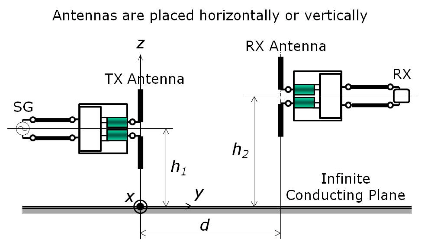
Fig. 1 shows the configuration of the SA measurement system using calculable dipole antennas with a 3-dB hybrid balun on the OATS. Two dipole antennas are located along the x-axis (horizontal polarization, HP) or the z-axis (vertical polarization, VP) above the ground plane with a TX antenna height of h1 and RX antenna height of h2. Further, d is the distance between the TX and RX antennas.
Normalized site attenuation measurement system.
Fig. 2 shows the power mismatch and dissipative loss factors of the SA measurement system and the basic structure of the CalDA. The balun was designed so that its complex S-parameters could be easily measured. Two semi-rigid cables with a length of LB from the 3-dB hybrid coupler are connected to the antenna terminal, as shown in Figs. 1 and 2. A 50-Ω load is connected to the sum port (∑) of the hybrid, and a matched measuring instrument is connected to the other port (Δ), using a coaxial cable with a length of L2. The inner conductors of the two semi-rigid cables are connected to the balanced dipole elements. Their outer conductors are in contact with each other electrically (i.e., short-circuited) at the feeding point of the dipole elements.

Normalized site attenuation measurement system using CalDAs. The CalDAs are placed horizontally or vertically.
The TX antenna is excited by a signal generator (SG), and the RX antenna receives the signal radiated by the TX antenna through the OATS, as shown in Fig. 2. The SA accounts for all power losses occurring between the RX and TX antennas over the ground plane. Two kinds of losses generally occur: conjugate mismatch losses and dissipative losses.
The CSA is defined as the minimum site power loss between the two antennas, including the baluns, as the RX antenna scans over a given height range. The CSA can be expressed in decibels in a simplified form [21]:
where
The expression of CSA can be evaluated by using impedance parameters of the TX and RX antennas. As shown in Appendix, the result is as follows:
Eq. (2) is the CSA expressed with antenna impedance parameters and balun impedances of the TX and RX parts. It is emphasized that Eq. (2) is a newly derived equation using the concepts of power mismatch and dissipative loss.
2. Normalized Site Attenuation
The theoretical NSA of an ideal OATS is defined as the normalized SA from CSA using AFs:
where AF1 and AF2 are the AFs for the TX and RX antennas, respectively. These include the mutual coupling effect between the ground plane and two antennas when TX and RX antennas are located for the measurement of the NSA. Note that the quantities in Eq. (3) are linear. All quantities in decibels appearing in the rest of the paper are given with (dB).
The theoretical NSA can be expressed in decibels as follows:
In relevant international standards, the theoretical NSA of an ideal OATS is defined as follows:
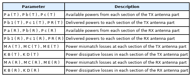
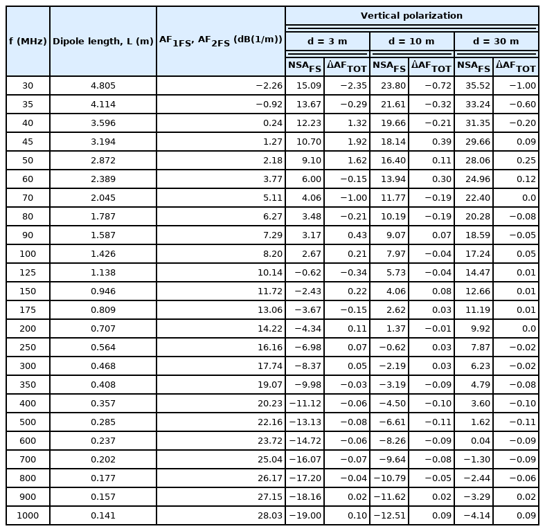
where AF1FS and AF2FS are the FSAFs of the TX and RX antennas, respectively. ΔAFTOT is the mutual impedance correction factor [1]. The relevant parameters for NSA calculation are listed in Table 1.

List of parameters for NSA calculation
3. Normalized Site Attenuation by Free-Space Antenna Factors
If we use FSAFs for measurements of the NSA, the mutual impedance correction factor is necessary. In this paper, the theoretical NSA by the FSAFs, SAFS, is normalized from the CSA by using the FSAFs.
Note that quantities in Eq. (6) are linear. In decibel form, Eq. (6) is expressed as follows:
In this case, an AF correction factor, ΔAFTOT, is necessary to obtain the true NSA, as shown in Eq. (5).
From Eqs. (5) and (7), the theoretical NSA of an ideal site is expressed as follows:
The difference between the true AF (AF1 and AF2) and the FSAFs (AF1FS and AF2FS) is expressed as follows:
Hence, the total AF difference is expressed as follows:
This is known as the mutual impedance correction factor that appears in Eq. (5) and the ANSI C63.4 standard [1].
Therefore, the difference between the true NSA and NSAFS is expressed as ΔNSA:
From Eqs. (4) and (7), ΔNSA is expressed as follows:
Therefore, the total mutual impedance correction factor ΔAFTOT is the same value as −ΔNSA.
4. Antenna Factors
In order to consider the theoretical NSA, the AFs of the TX and RX antennas, AF1 and AF2, are needed to calculate the NSA. Fig. 3 shows the TX and RX antennas for the evaluation of the AFs. Note that the power loss parameters of the TX antenna part in Fig. 3(a) are different from those in Fig. 2 because the AF is defined in the receiving mode. To unify the AF representation, the TX and RX parts are represented by the superscripts T and R, respectively. For the RX part, Fig. 3(b) is the same as Fig. 2—i.e.,

TX and RX antennas for calculation of AFs: (a) TX antenna and (b) RX antenna.
The details of the CalDA analysis using the power mismatch and dissipative loss concepts are given in other studies [19, 20]. The desired AFs of the TX and RX antennas above a ground plane, AF1(h1, h2, d) and AF2(h1, h2, d), can be expressed as follows:
where
List of parameters for AF calculation
where
Since the hybrid balun has a 100-Ω balanced port and a 50-Ω unbalanced port [19],
The true AF1 and AF2 values are different from the FSAFs (AF1FS and AF2FS). The AF1 is also different from the AF2 because the height of the TX antenna is fixed, but the RX antenna’s height is scanned above the ground plane.
As shown in Eqs. (9) and (10), the total AF difference between the true AF and the FSAF is expressed as follows:
The total AF difference ΔAFTOT corresponds to the total AF correction factor and is known as the mutual impedance correction factor, as explained in Section II-3.
III. Numerical Results and Discussions
1. Normalized Site Attenuation
In the calculation of the theoretical NSA of an ideal OATS from Eqs. (3), (13), and (14), the TX and RX antenna system analysis is required, in which case a thin-wire kernel approximation with a segment length of 0.0125λ is used for the piecewise sinusoidal Galerkin’s methods of moment analysis, as presented in [19–21]. The dipole radius (α = 3.175 mm; 30 MHz ≤ f < 300 MHz and α = 0.794 mm; 300 MHz ≤ f ≤ 1 GHz ) was chosen to be less than 0.007λ (thin-wire approximation). A nominal value of 50 Ω was used for the characteristic impedance Z0. A coaxial cable (RG-214/U) with a length of 10 m was selected for the numerical calculation (the velocity of propagation is 66% of the velocity in free space, and the dielectric constant ɛr is 2.3). Fig. 4 shows the frequency characteristics of the calculated theoretical NSA from Eq. (3) for the horizontal and vertical polarizations at given distances of 3 m, 10 m, and 30 m. The detailed values of the theoretical NSAs calculated in this paper are shown in Table 3. In these tables, the resonant dipole lengths for a CalDA with a 3-dB hybrid balun in the frequency range of 30 MHz to 1 GHz are shown for 24 individual frequencies. The height of the RX antenna when measuring the CSA at the given distances is also shown. These theoretical NSA values (Fig. 4, Table 3) were used as reference theoretical NSA values for the validation test of an OATS or a semi-anechoic chamber using the CalDAs.
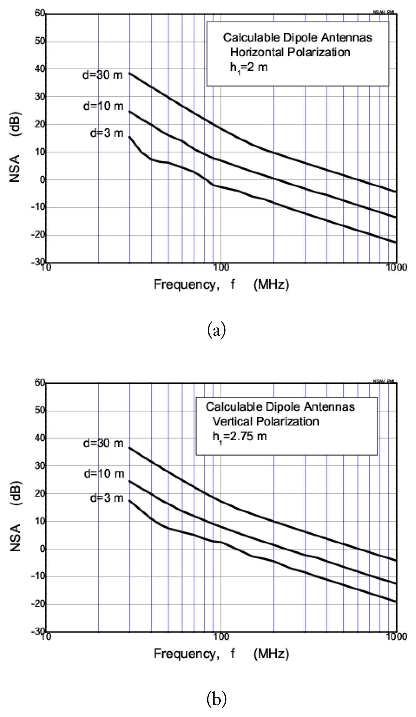
Calculated site attenuations for (a) horizontal polarization and (b) vertical polarization.
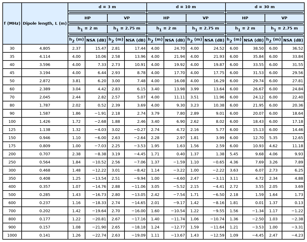
Calculated NSA for 3 m, 10 m, and 30 m
2. Antenna Factors
Tables 4 and 5 show the AF1, AF2, and CSA values calculated from Eqs. (13) and (1). For example, a CSA of 13.34 dB is obtained when h1 = 2 m and h2 = 1.72 m with d = 3 m, H-polarization, and f = 100 MHz. In this case, TX and RX AFs are AF1(2 m) = 8.15 dB(1/m) and AF2(1.72 m) = 7.87 dB(1/m), respectively. From these CSAs, AF1, and AF2, the theoretical NSA from Eq. (4) is calculated as −2.68 dB. The resulting NSA values for 24 individual frequencies are shown in Fig. 4 and Table 3. Tables 4 and 5 are also useful for checking the AFs (AF1 and AF2) above the ground plane giving the NSA.

Calculated CSA (dB) and AF (dB(1/m)) for horizontal polarization

Calculated CSA (dB) and AF (dB(1/m)) for vertical polarization
In general, AFs provided with the antenna are inadequate unless they are specifically or individually measured and the calibration is traceable to a national standard. In an actual validation test, the use of the AFs above the ground plane is inadequate because individual AF calibration at a given antenna height above the ground plane is needed, and this procedure is inefficient. For this reason, the FSAFs for the TX and RX antennas were used to determine the NSA measurements.
3. Normalized Site Attenuation by Free-Space Antenna Factors
ANSI C63.5 gives the FSAFs for a tuned dipole with a Roberts balun. Tables 6 and 7 show the theoretical FSAFs for a CalDA. A comparison of both FSAFs, the Roberts dipole and the CalDA, is not adequate because the dipole radius, resonant lengths, and balun types are different. Nevertheless, the FSAF differences between both antennas are within 0.56 dB.

Calculated NSAFS using the FSAFs and AF correction factor in dB for horizontal polarization
Calculated NSAFS using the FSAFs and AF correction factor in dB for vertical polarization
In a relevant standard, the theoretical NSA of an ideal OATS is developed and calculated using FSAFs and mutual impedance correction factors. ANSI C63.4 [1] provides theoretical NSA values and mutual impedance correction factors for the tuned dipoles with a Roberts balun and a 3-m site. When the theoretical NSA from FSAFs, NSAFS, is used for the NSA measurement using the CalDA, the measured NSAs are different from the true NSA. Hence, ΔAFTOT for the CalDA is necessary.
Tables 6 and 7 show the calculated NSAFS from the FSAFs of the TX and RX antennas and the mutual impedance correction factors ΔAFTOT for the CalDA. ΔAFTOT is calculated from Eq. (16) and is known as the total AF difference, as explained in Section II-3. Hence, the FSAFs, AF1FS and AF2FS, are used to measure the NSA. Further, the mutual impedance correction factor, ΔAFTOT, is provided to obtain the true NSA. For example, the NSAFS of −3.06 dB is obtained from the CSA of 13.34 dB using the free space, AF1FS, of 8.20 dB(1/m) at d = 3 m, H-polarization, and f = 100 MHz. In this case, the mutual impedance correction factor, ΔAFTOT, is necessary, and from Table 6, since ΔAFTOT = −0.38 dB, the desired NSA = −2.68 dB is obtained from Eq. (8). Tables 6 and 7 are useful for actual NSA measurement, using the FSAFs and the mutual impedance correction factors of the CalDA.
To validate a constructed site, the true theoretical NSA values are very important as a reference, and the measured NSA should be within ±4 dB. The use of AFs over the ground plane is inadequate because the AF calibration for an individual height over the ground plane is very hard and time consuming. Hence, the use of FSAFs is recommended for easy AF calibration and to save time. Consequently, we considered the true theoretical NSA of an ideal OATS, the FSAFs, and the AF correction factors (mutual impedance correction factors) for a CalDA and for 3-m, 10-m, and 30-m sites.
In order to calculate the NSA, the CSA and AFs are needed. To verify these theoretical analyses, the theoretical results of CSA and AF are compared with the experimental results [16, 17] in Figs. 5 and 6. The AF is measured by the two-antenna method. The results show that the calculated CSA and AF values are in good agreement with the measured results.
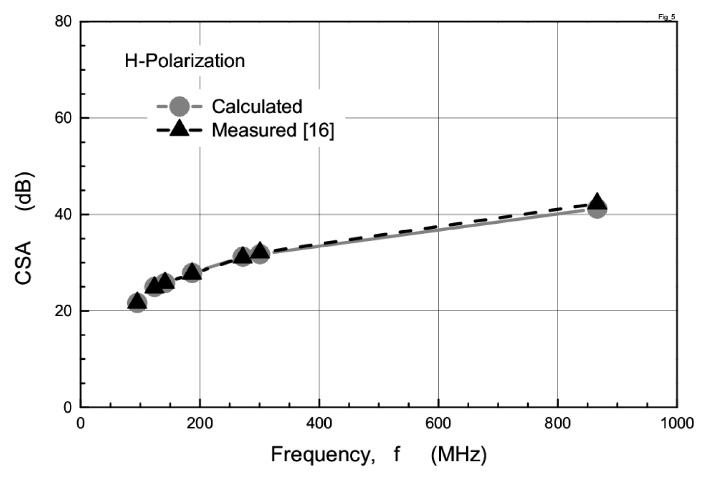
Calculated and measured site attenuations.
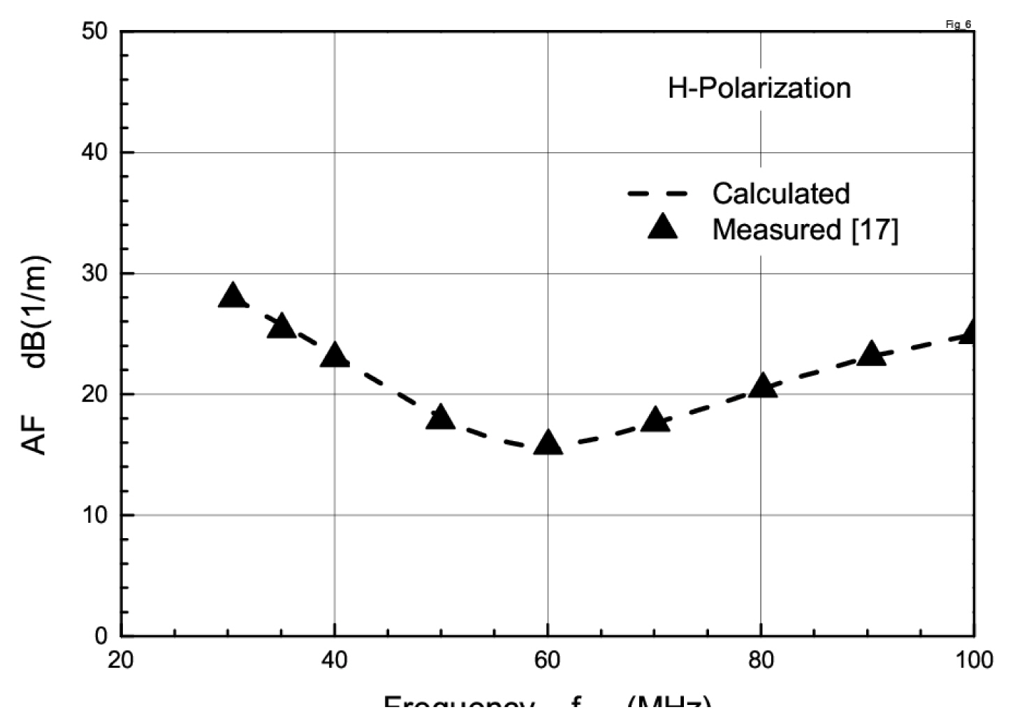
Calculated and measured antenna factors.
IV. Conclusion
The theoretical NSA values of an ideal OATS for a CalDA with a 3-dB hybrid balun in the frequency range of 30 MHz to 1 GHz were considered using the power mismatch and dissipated loss concept of an NSA measurement system. We also considered the accurate AFs above the ground plane to obtain the theoretical NSA. In addition, when the FSAFs were used to determine the measured NSA, the AF correction factors for the CalDAs were also considered.
Acknowledgments
This work was initially based on the KRISS/University cooperative research program. It was supported by the Basic Science Research Program at the National Research Foundation of Korea (NRF), funded by the Ministry of Education (No. 2021R1I1A3053429).
References
Appendices
Appendix
The CSA of Eq. (1) is determined by the antenna input impedance
The desired CSA can be written as follows [21]:
where power mismatch and dissipative losses using the impedance parameters are expressed as
Using Eqs. (A2)–(A4), the CSA is obtained:
Therefore, the desired CSA by means of the impedance parameters of the antenna system can be expressed in dB as follows:
Biography

Ki-Chai Kim received his B.S. degree in electronic engineering from Yeungnam University, Korea, in 1984, and M.S. and Ph.D. degrees in electrical engineering from Keio University, Japan, in 1986 and 1989, respectively. He was a senior researcher at the Korea Standards Research Institute, Daedok Science Town, Korea, until 1993, working in electromagnetic compatibility. From 1993 to 1995, he was an associate professor at Fukuoka Institute of Technology, Fukuoka, Japan. Since 1995, he has been with Yeungnam University, Gyeongsan, Korea, where he is currently a professor in the Department of Electrical Engineering. He received the 1988 Young Engineer Award from the Institute of Electronics, Information and Communication Engineers (IEICE) of Japan as well as the Paper Presentation Award in 1994 from the Institute of Electrical Engineers (IEE) of Japan. Prof. Kim served as president of the Korea Institute of Electromagnetic Engineering and Science (KIEES) in 2012. His research interests include EMC/EMI antenna evaluation, electromagnetic penetration problems in slots, and the applications of electromagnetic fields and waves.

Hyuk-Jun Seo received his B.S. degree in electronics and computer engineering from Kyungpook National University, Daegu, Korea, in 2006, M.S. degree in engineering science from the University of Mississippi, MS, USA, in 2010, and Ph.D. degree from Yeungnam University, Gyeongsan, Korea, in 2022. From 2011 to 2013, he was a junior research engineer at the Mobile Communication Advanced Product Research Institute of LG Electronics Inc., Seoul, Korea. Since 2014, he has been a research engineer at the Medical Device Development Center, Daegu-Gyeongbuk Medical Innovation Foundation (K-MEDI hub), Daegu, Korea. His research interests include the design areas of EMC/EMI antennas, EMC test standards, and the validation of the test site.

Tae-Weon Kang received his B.S. degree in electronic engineering from Kyungpook National University, Daegu, Korea, in 1988 and M.S. and Ph.D. degrees in electronic and electrical engineering from Pohang University of Science and Technology (POSTECH), Pohang, Korea, in 1990 and 2001, respectively. Since 1990, he has been with the Korea Research Institute of Standards and Science, Daejeon, Korea, working on electromagnetic metrology as a principal research scientist. He spent the year 2002 as a visiting researcher as part of the Korea Science and Engineering Foundation postdoctoral fellowship program at the George Green Institute for Electromagnetics Research, University of Nottingham, UK, and he worked there on the measurement of the absorbing performance of electromagnetic absorbers and on a generalized transmission line modeling method. His research interests include electromagnetic metrology, such as power, noise, RF voltage, impedance, field strength, and standardization of electromagnetic compatibility, including test methods and characterization of measuring instruments. He is an associate editor for the journal IEEE Transactions on Instrumentation and Measurement and an IEEE senior member. He received the Outstanding Researcher Award from the Korean Institute of Electromagnetic Engineering and Science (KIEES) in 2017.

Jae-Yong Kwon received his B.S. degree in electronics from Kyungpook National University, Daegu, in 1995, and his M.S. and Ph.D. degrees in electrical engineering from the Korea Advanced Institute of Science and Technology, Daejeon, Korea, in 1998 and 2002, respectively. He was a visiting scientist at the Department of High-Frequency and Semiconductor System Technologies, Technical University of Berlin, Berlin, Germany, and at the National Institute of Standards and Technology (NIST) in Boulder, CO, USA, in 2001 and 2010, respectively. From 2002 to 2005, he was a senior research engineer at the Devices and Materials Laboratory, LG Electronics Institute of Technology, Seoul, Korea. Since 2005, he has been a principal research scientist with the Division of Physical Metrology, Center for Electromagnetic Metrology, Korea Research Institute of Standards and Science, Daejeon. Since 2013, he has been a professor of the science of measurement at the University of Science and Technology, Daejeon. His current research interests include electromagnetic power, impedance, and antenna measurement. Dr. Kwon is an IEEE senior member and an IEICE member.

Jeong-Hwan Kim was born in Cheongju, Korea, in 1954. He received his B.S. degree in electrical engineering from Seoul National University, Seoul, Korea, in 1978 and his M.S. and Ph.D. degrees from Korea Advanced Institute of Science and Technology, Seoul, Korea, in 1980 and 2000, respectively, both in electrical and electronic engineering. He joined the Center for Electromagnetic Wave of the Korea Research Institute of Standards and Science, Daejeon, Korea, in 1981. Since then, he has been working on the development of six-port automatic network analyzer systems, standard antennas, and electromagnetics measurement standards. Dr. Kim is currently a technical advisor at the Institute of Calibration & Technology Co. Ltd.