Time Domain Signal Simulation of Weather Clutter for an Airborne Radar Based on Measured Data
Article information
Abstract
An airborne radar simulator for an X-band radar echo signal was implemented and numerically verified. The simulator can consider weather conditions over a large area and can use measured S-band data as input. A scheme is presented for the conversion of the S-band data to the X-band one. The amplitude and time delay due to weather particles can be theoretically calculated on the basis of reflectivity. The dynamics of the platform and clutter particles were modeled using the Doppler frequency shift in the echo signal. As the simulated weather area was very large, an efficient approximation method was designed for use in calculating the attenuation and time delay, which was also numerically verified. Finally, a scheme for extracting the reflectivity from the echo signal was formulated and was verified by comparing it with the input data.
I. Introduction
Airborne radar modeling and simulation (M&S) methods have been developed and used for decades, especially in military research. One reason for this is that obtaining real field data is difficult and not economically efficient [1–3]. For the wide application of M&S techniques, sophisticated and accurate simulation data are required, which might include echo signals from not only a target but also radar clutter.
There are many types of radar clutter, such as surface or volume clutter from objects such as forests, vegetation, lakes, and weather particles. Among these, weather clutter is usually distributed over a wide area, and its properties are strongly dependent on weather conditions or types of weather particles, such as rain, snow, and hail. At a higher radar frequency, the echo signal is strongly affected by weather conditions, which may be attenuated or delayed in the time domain [3–5]. Therefore, estimating the effect of various weather conditions on the echo signal is important for radar M&S techniques.
In general, weather conditions are continuously monitored by many ground-based weather radars throughout the world. One example of a ground-based weather radar is NEXRAD, which is operated by the National Weather Service (NWS) and the National Oceanic and Atmospheric Administration. The operating frequency of the ground-based radar is the S-band. The measured data are available to the public [6–9] and are categorized into three levels.
The Level I data are raw time series I and Q data. The Level II data consist of some processed data from Level I data, such as reflectivity (ZH,V) and mean radial velocity. The Level III data are more processed data, such as hydrometeor classification, instantaneous precipitation, and tornadic vortex signature [6, 8]. Among these three-level datasets, Level II data can be used for the generation of echo signals.
The X-band frequency has become popular of late for airborne radars, but the available measured weather data in this band are very limited. In addition, to estimate the minute dynamics of the target or clutter, micro-Doppler techniques have been studied [10]. Therefore, to simulate an X-band radar echo signal, weather data are numerically generated by a numerical weather prediction code or converted from the available S-band data [11, 12].
A computational scheme is proposed to generate an echo signal on the basis of the measured S-band data. First, the data transformation from the S-band to the X-band is addressed in Section II. Then the signal calculation scheme is explained. In Section III, a method of extracting reflectivity from the generated signal is proposed, and its numerical verification is presented.
II. Time Domain Signal Generation
1. Weather Data Preparation
Ground-based radar data are collected in spherical coordinates centered at the radar, and their range resolution is 250 m. The operating frequency of the radar is the S-band (2.8 GHz), and its polarization is horizontal polarization (h-pol). Data from the radar located in Gunsan, Korea, were used in this study. The data were collected at 00:05 on 08/11/2020. We adopted the Level II data in the measured dataset, which included the h-pol reflectivity (ZH ), differential reflectivity (ZDR =ZH − ZV), radial wind velocity, and wind spectral width, as summarized in Table 1 [13, 14]. The subscripts H and V indicate the h-pol and vertical polarization (v-pol), respectively. The v-pol reflectivity is calculated as ZV =ZH − ZDR.
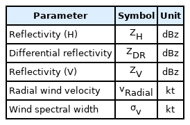
Weather parameters for simulation
We generated an X-band airborne radar echo signal on the basis of the measured S-band data. Therefore, data conversion from the S-band to the X-band was required. As reflectivity is generated by many small weather particles, such as rain droplets, it may be dependent on the radar frequency. However, on the basis of known experiments and simulations [12, 15], the ratio of the reflectivity for the S-band to that for the X-band is almost unity. It can thus be directly adopted for X-band simulation without conversion. To partially consider the shape of the weather particles, we considered the canting angle effect, which could improve the accuracy of the other required quantities, such as the phase shift.
Radial wind velocity is the kinetic quantity of the weather particles, which might be independent of the radar frequency [13]. Hence, reflectivity and radial wind velocity can be directly used for X-band simulation. As the wind spectral width (σv) is related to the dynamic of the weather clutter, it is also independent of the frequency. However, it determines the spread of the Doppler spectrum (σf) of the echo signal [16], which is dependent on the radar frequency:
where λ is the wavelength of the radar signal.
2. Three-Dimensional Clutter Model and Simulation Scenario
Fig. 1 shows the simulation geometry and antenna coordinates that were used. The entire weather area was modeled by a large box that was discretized into many smaller sub-boxes. Each box represented a different weather clutter at a specific point, and the properties were assumed to be uniform over a sub-box. The measured data were assigned to the center of the sub-boxes.
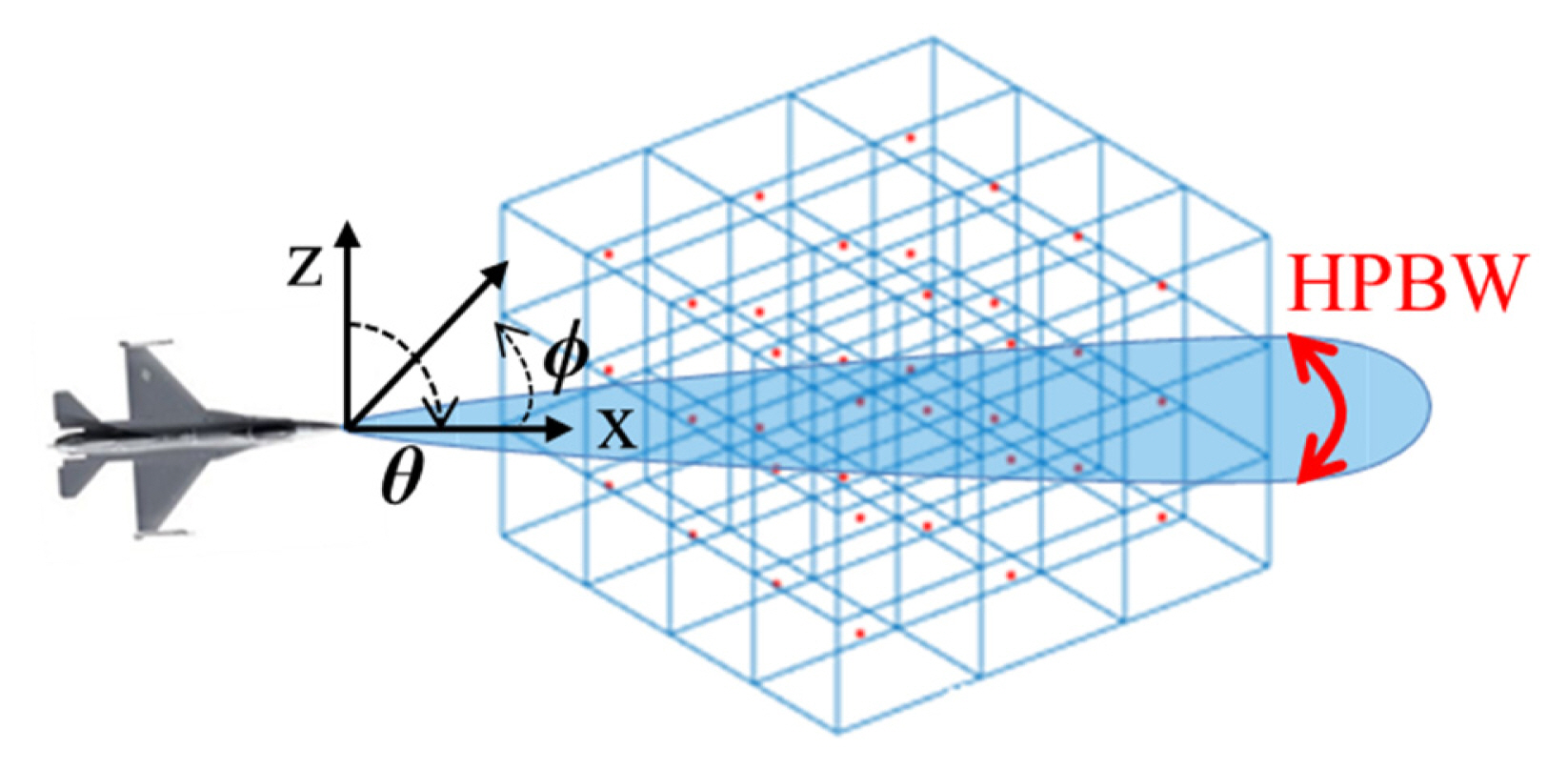
Simulation scenario and three-dimensional weather clutter model.
The airborne radar beam scans in the horizontal (azimuth) direction, with a fixed elevation angle and a v-pol wave. Four pulses were transmitted to measure the weather conditions at each azimuth direction. The range resolution of the NWS data was 250 m, but the size of the small box was set at 125 m to improve the final signal accuracy and to simulate a large weather area covering dozens of kilometers. In one horizontal scan, the boxes inside the half-power beam width (HPBW) of the radar antenna were selected to generate the return signal.
The return impulse’s location in the time domain could be precisely calculated using the distance between the radar and the sub-box centers, which would be slightly perturbed due to the weather particles. The amplitude of the impulse was calculated using the radar equation based on the given reflectivity. For the simulations in this study, the radar was located at (0, 0, 3) km in Cartesian coordinates. The center point of the clutter box was (20, 0, 3) km, and its dimensions were 30 km × 0.5 km × 0.5 km.
Fig. 2 shows the mean, maximum, and minimum values of the measured data of the sub-boxes in the identical range bin for θ = 90° and φ = 0°. The vertical line shows the maximum and minimum values in a range bin. The data were spread within a wide range.
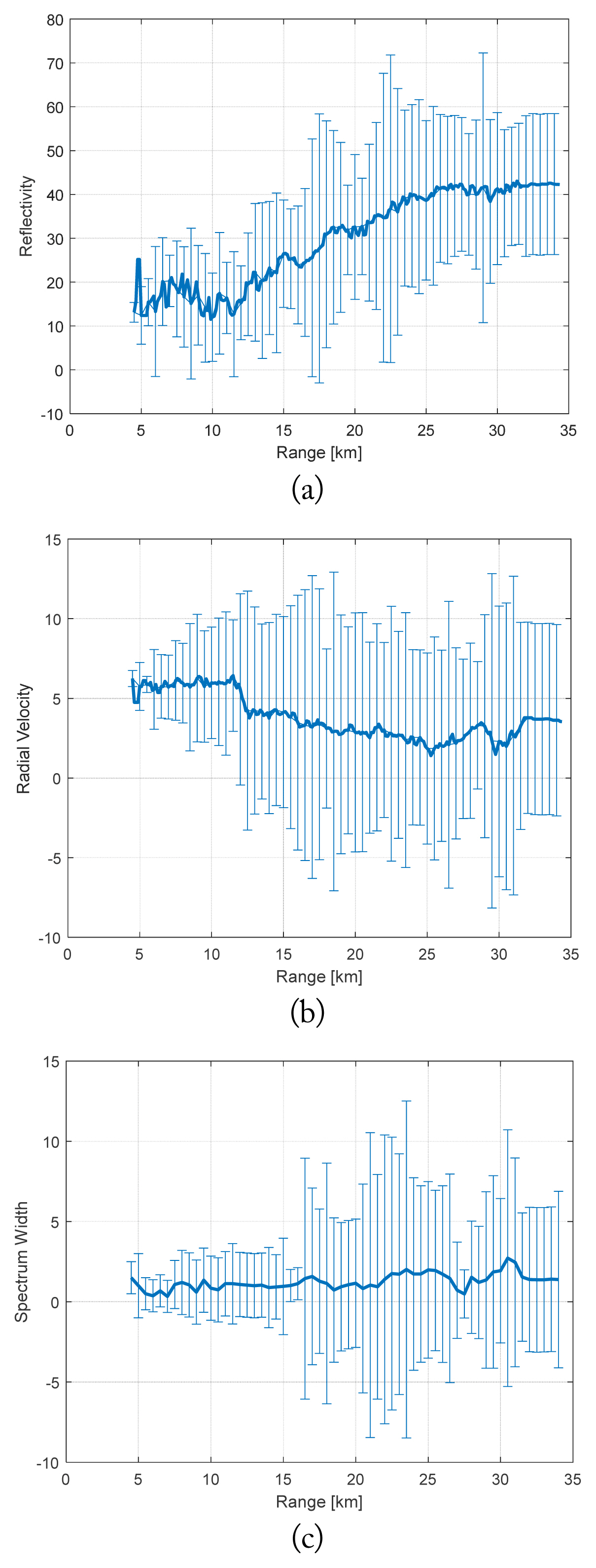
Mean, maximum, and minimum values of the weather data in each range resolution bin. (a) Reflectivity, ZV (dBz). (b) Wind radial velocity, vRadial (m/s). (c) Wind spectral width, σv (m/s).
3. Signal Amplitude and Attenuation
The amplitude of the impulse from each box could be independently calculated with the assigned properties of the box using the radar equation, as follows:
where Pt, Pr, and G are the transmitted power, received power, and antenna gain, respectively; R is the range from the radar to each box center; σ is the range from the radar to the radar cross-section (RCS) of the box (expressed as ηdV); dV is the volume of the sub-box; and η is the RCS per unit volume, which is directly related to reflectivity [13], as follows:
where K is a complex dielectric constant [17]. Therefore, the signal amplitude could be formulated as follows:
Due to the randomness of the weather clutter, the return signal was also random. A Gaussian distribution was assumed over the pulses, and the mean and variance were assumed to be 0 and
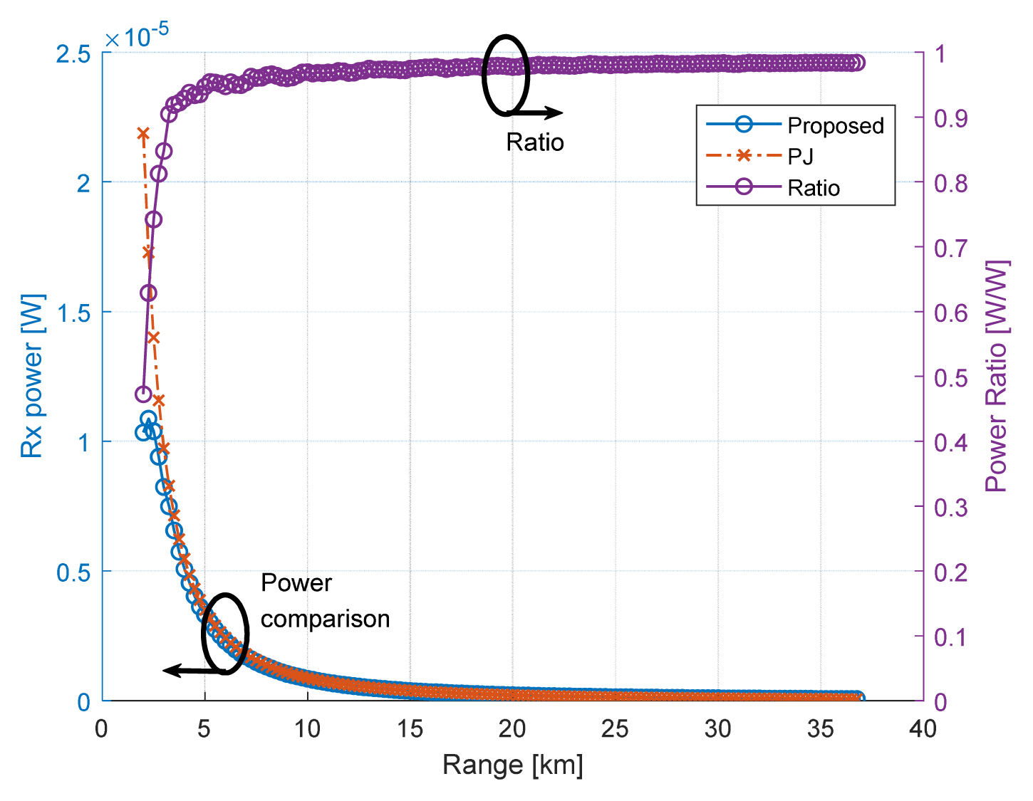
Comparison of the power ratios of the proposed scheme and of the PJ equation.
The power ratio of Eq. (4) to the PJ equation is shown in Fig. 3. It approaches 1 as the range profile increases. In the short range, some discrepancies can be observed due to the difference between the volume of the box for Eq. (2) and the volume of the cylinder for the PJ equation in a range bin. However, the discrepancies quickly decreased over the range profile.
Due to the particles inside the weather clutter, the signal is attenuated as it propagates through the clutter. For long-range propagation, the attenuation effect may be significant, especially in the X-band [18, 19]. The weather clutter was highly inhomogeneous, so the attenuation was strongly dependent on the signal path inside the clutter. Estimating the exact path length over many small boxes is very time consuming. Therefore, we approximated the exact path length as the size of a box, dL = 125 m, which resulted in a very small attenuation error for a sub-box.
The specific attenuation (γR) of a sub-box recommended by the ITU Radiocommunication Sector (ITU-R) is as follows:
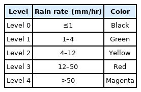
where r is the rain rate in mm/hr and κ and α are constants equal to 0.008853 and 1.2636, respectively, for the X-band and v-pol. The rain rate can be estimated on the basis of the reflectivity and weather clutter type shown in Table 2, which are given by the NWS and a previous study [20]. Thus, the attenuation for the round trip was approximated as follows:
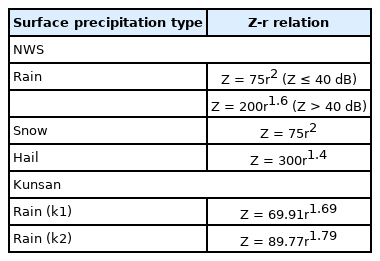
Relation between reflectivity and rain rate
where R0 and R1 are the start and end ranges of the clutter, respectively. Finally, the value obtained from Eq. (6) was multiplied by the value obtained from Eq. (4) for each impulse.
4. Time Delay (Phase Shift)
The weather particles also decrease the signal velocity, which results in time delay and phase shift in the time and frequency domains, respectively, as shown in Fig. 4. We analytically calculated the phase shift and then converted it to the time delay. The frequency shift can be calculated as follows [21]:
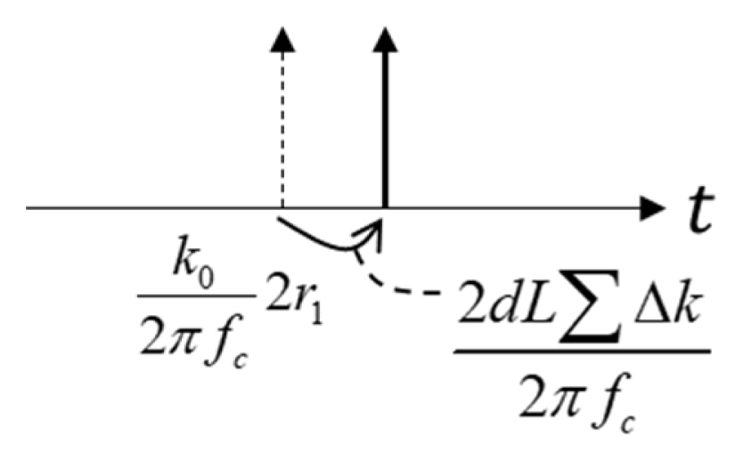
Time shift description converted from phase shift.
where N0, αk, and βk are constants based on the type of clutter [22]; Γ(·) is the Gamma function; and Λ is a slope parameter related to reflectivity ZV, as follows:
where αb, βb, αa, and βa are constants dependent on the clutter type [17, 22] and A, B, and C are related to the canting angle effect and describe the hydrometeor’s orientation [21, 22]. The canting angle effect is more important for the X-band than for the S-band due to the shorter wavelength. Using Eq. (8), Λ can be estimated by considering the frequency property of the radar, and then Δk can be computed using Eq. (7). The overall phase shift can be approximated as follows:
The phase shift (9) is directly converted to the time delay, as follows:
where fc is the carrier frequency [23, 24]. Fig. 5 compares the exact and approximated estimations of the time delay and attenuation, which are cumulatively calculated values along the line-of-sight (LOS) for θ = 90° and φ = 11.6°.
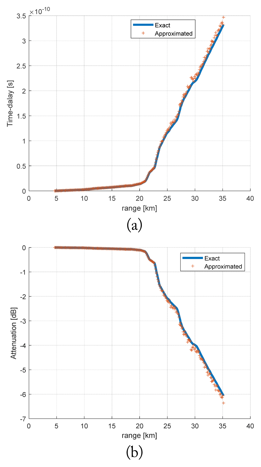
Comparison of time delay and attenuation calculated using the proposed approximate and exact methods for the LOS direction, θ = 90° and φ = 11.6°. (a) Time delay. (b) Attenuation.
5. Time Domain Signal
The echo impulse responses from many sub-boxes in an identical range bin (Δr) are coherently integrated. Fig. 6 shows the generated time domain signal for the input data in Fig. 2. It shows the magnitude of the one-dimensional (1D) signal with and without an attenuation effect for rain clutter. As expected, the amplitude of the signal is proportional to the reflectivity in Fig. 2(a).
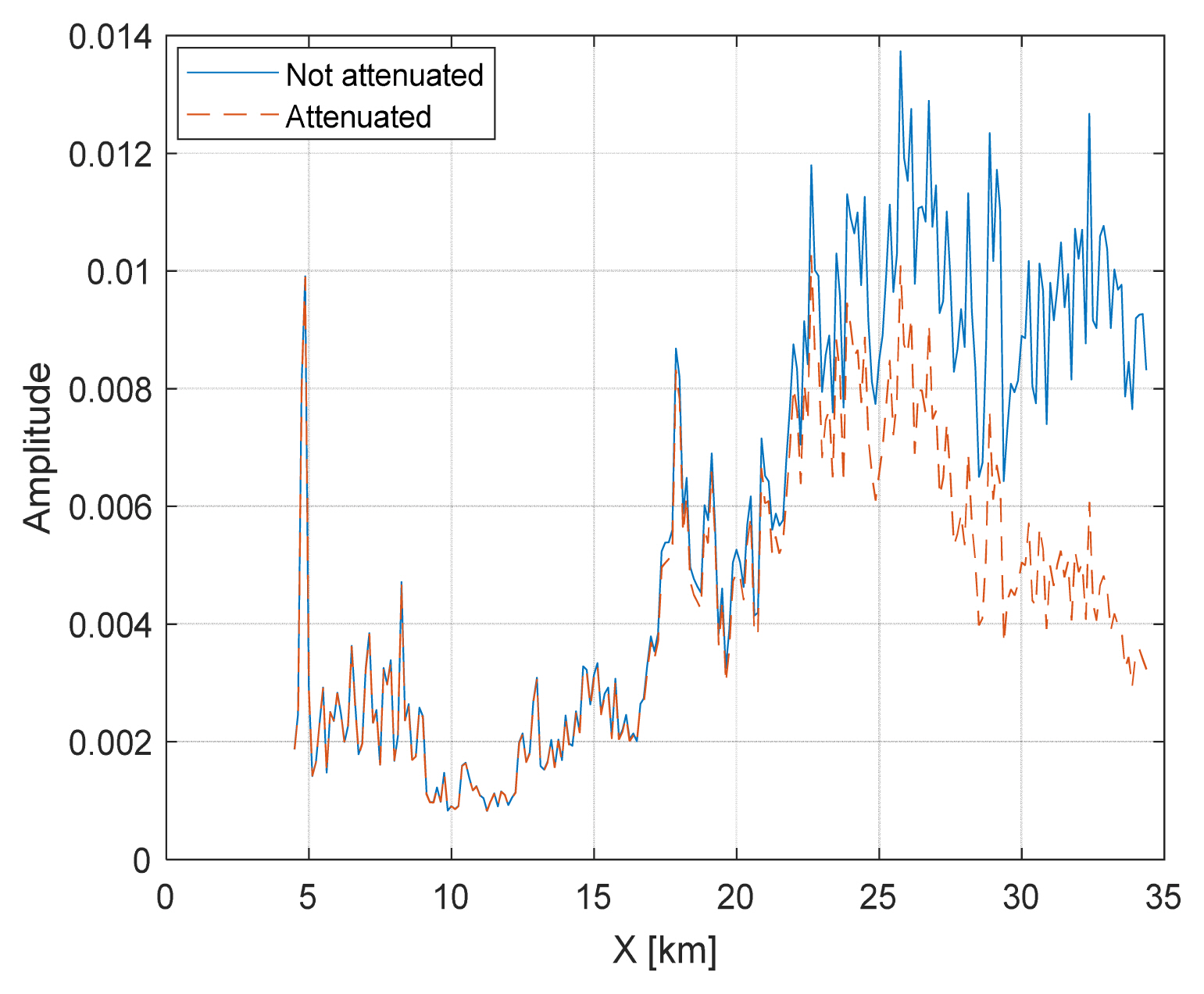
Magnitude of one-dimensional time domain signals with and without an attenuation effect.
Due to the dynamics of the platform and clutter particles, successive pulses are slightly distorted and can be modeled using the Doppler frequency shift. The power spectrum density of the Doppler frequency can usually be assumed to be a Gaussian probability density function (PDF) [16], given by:
where σf is calculated using Eq. (1) and fD is the mean Doppler frequency of the clutter related to the radial wind velocity. Eq. (11) is converted to the correlation between the pulses in the time domain, which is also written in terms of the Gaussian function with the assumption of fD= 0, as follows:
where n and Ts are the indices of the pulse and the pulse repetition interval, respectively. The correlating Gaussian random variable can be generated through the Cholesky decomposition method and the mean Doppler frequency in Fig. 2(b), and the platform velocity is consecutively applied to the signal, as described in other studies [16, 25].
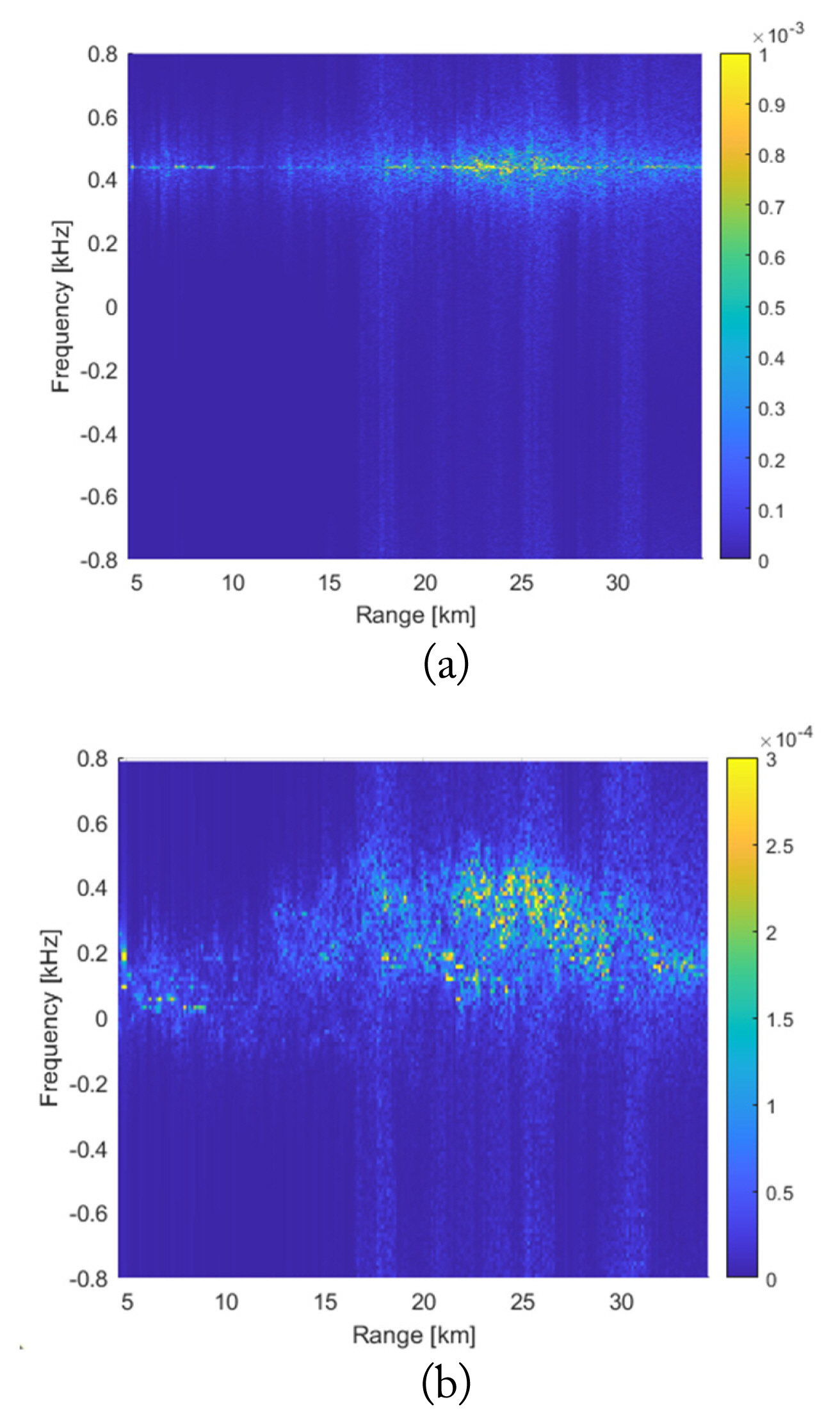
The accuracy of the Doppler shift can be examined on the basis of the range-Doppler (RD) maps. To generate a fine RD map, 256 pulses were transmitted and processed for the situation in Fig. 6, with an attenuation effect. Fig. 7 shows a simulated RD map with a 180 m/s flight velocity toward the positive x-axis. In the calculation for Fig. 7(a), only the flight Doppler effect was included (the wind effect was not included). From the RD map, the peak Doppler shift is around 444 Hz, which can be converted to 179.4 m/s. This agrees well with the 180 m/s flight velocity. In Fig. 7(b), the wind effect is included. The radial velocity of the wind in each sub-box is also applied with the flight velocity to the signal, which decreases the peak frequency if the wind direction is identical to that of the flight. Hence, the Doppler frequency is decreased, as shown in Fig. 7(b). Beyond 12 km, the mean wind velocity decreases, and beyond 20 km, it increases. Thus, the Doppler frequency decreased beyond 12 km and increased again beyond 20 km. Over the 20–25 km region, the Doppler frequency was distributed over 50–500 Hz on the RD map, which is attributed to the variance of the wind radial velocity in Fig. 2(b) for each sub-box at 20–25 km (−1 to 6 m/s). This velocity could be converted to −388 to 64 Hz and was added to the flight Doppler frequency of 444 Hz. Then, it became 56–508 Hz, which is very similar to the estimated variation in the RD map (50–500 Hz).
III. Reflectivity Estimation
To simulate the weather map, reflectivity ZV should be extracted from the generated two-dimensional (2D) signal. Then the weather map was constructed from the rain rate using the colors in Table 3. The amplitude of the 1D signal at a time point might be random because it is affected by the reflectivity of many sub-boxes inside the identical range bin. Due to the central limit theorem, the amplitude can be approximated using a Gaussian PDF. Hence, an estimator of reflectivity was developed on the basis of the Gaussian PDF assumption. The signal amplitude in a range bin is the summation of Eq. (4) over the sub-boxes, as follows:
Weather map color definition with rain rate
where Nc is the number of sub-boxes in a range bin. The constants Pt, λ, π, K, and dV can be simply removed by dividing them out from the received signal.
The antenna gain Gk and the range between the radar and each box Rk are different for each box. Only the boxes inside HPBW were considered, and all were in the far-field region. Thus, the gain and distance could be approximated by the mean gain and distance (Rmid) of all the sub-boxes and were removed. After this algebraic manipulation, Eq. (13) was reduced to the following:
where X is a Gaussian random variable. The reflectivity was inhomogeneous and could be assumed to be independent of the sub-boxes due to the large box dimension (125 m). Therefore, the following could be obtained [26]:
Finally, by taking the expectation, E[·], the estimator of reflectivity can be formulated as E[X2]. To compute the reflectivity for a box, we divided E[X2] with the box number estimated using the assumption that the volume was an elliptical cylinder [13, 14].
Fig. 8 shows the estimated reflectivity from the generated 2D signal with and without an attenuation effect for the simulation case in Fig. 6. The estimation result was compared with the mean input reflectivity in each range bin. The two results were in excellent agreement, but if the attenuation effect were included, the discrepancy would become larger with increasing range.
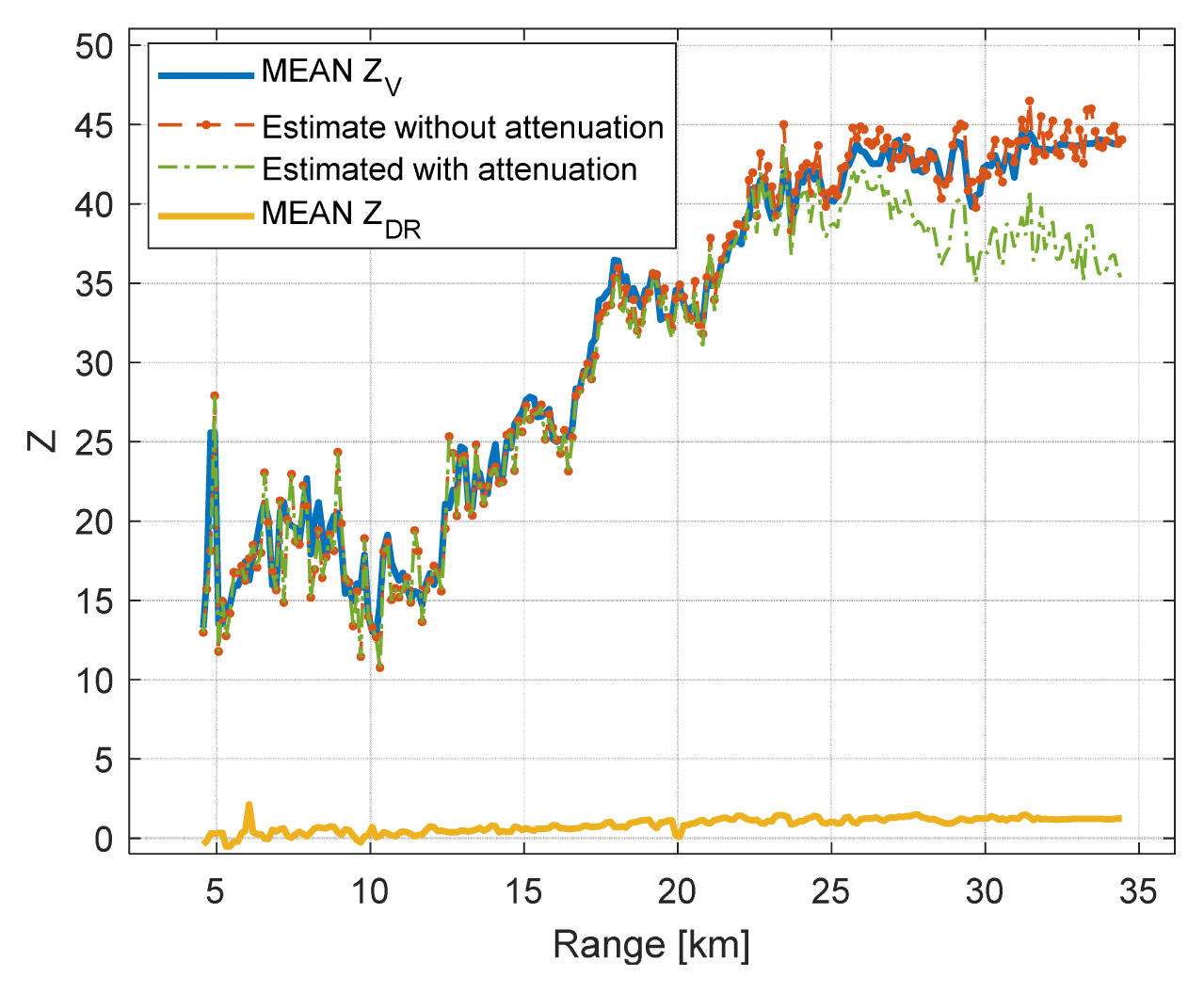
Fig. 9 shows the weather maps extracted from the 2D signal and the input data, which also agree well. The weather map from the input data was calculated from the mean reflectivity inside the identical range bin. For this simulation, seven azimuth angles, from −11° to 11°, were scanned. The attenuation effect decreased the reflectivity from around 20 km, and the reflectivity was reduced by 10 dB compared with that for the S-band at 35 km. These results agree well with the previous simulation results [15].

Weather map generated by seven azimuth boresight angle sweeps from −11° to 11° using input data (a) and the estimated Z-parameter (b).
For a final verification, we compared the estimated rain rate with the instantaneous rain rate in the Level III data. The Level III data were processed by the data provider through the dual polarization measurement, and the azimuth resolution was different from that of the Level II data: the instantaneous rain rate was given every 1°. Hence, three instantaneous rain rates along the azimuth range were averaged for comparison with the estimation results.
For the aforementioned comparison, rain clutter was assumed. Three rain rates were computed from the reflectivity estimated using the NWS equation, and were denoted as “Estimated.” Two equations were used to fit the Kunsan region data [20], and the results were denoted as “Estimated-k1” and “Estimated-k2,” respectively, in Fig. 10. The explicit equations are given in Table 2. The Z-r empirical relation is generally developed on the basis of the ZH parameter; thus, the rain rate estimated using ZH is also shown in Fig. 10. The two estimated reflectivities are shown in Fig. 8.

Comparison of the rain rate from Level III data and the estimated rates for both v-pol and h-pol (increased by 50 dB).
ZDR was around 1.2 dB; thus, the two estimated rain rates were very similar, but the h-pol estimation was slightly more accurate. The Z-r empirical relation processed on the basis of the Gunsan data could provide more accurate results, while the NWS one, which was developed with US region data, was less accurate. Accordingly, the generated 2D signal can be used for a radar simulation, considering the weather conditions.
IV. Conclusion
A calculation scheme was proposed for the generation of a 2D time domain radar echo signal from a large-volume weather clutter in the X-band. Measured Level II data were utilized. As the dataset was measured in the S-band, the data were converted to X-band data. The entire weather area was modeled by a large box discretized into many small boxes. Weather data were assigned to each box center.
Reflectivity was used to compute the specific phase shift and attenuation of the radar signal, as recommended by ITU-R and a known analytical formulation. As the canting angle effect was partially considered, several types of weather clutter could be simulated, such as rain, snow, fog, and hail. The received power and Doppler frequency shift were validated by comparing them with those obtained using known formulations, such as the PJ equation and RD map.
An estimator of reflectivity that could be used to extract the reflectivity from the received signal was proposed, and it was verified by comparing the estimated value and the input data. In addition, a weather map was generated on the basis of the estimated reflectivity, which had excellent agreement with the result based on the input data. The rain rates were calculated and compared with the instantaneous rain rate among the Level III data. The rain rates were computed using three Z-r empirical relations. Their comparison showed that the generated 2D signal could provide accurate results.
Acknowledgments
This work was supported by a grant-in-aid from Hanwha Systems.
References
Biography

Jihyo Choi received B.S. and M.S. degrees in electronic engineering from Inha University, Incheon, Korea, in 2020 and 2022. She is currently a junior engineer at Hanwha Systems, Gyeonggi-do, Korea. Her research interests include radar system modeling and radar clutter signal modeling and analysis.

Il-Suek Koh received B.S. and M.S. degrees in electronics engineering from Yonsei University, Seoul, Korea, in 1992 and 1994, respectively, and a Ph.D. from the University of Michigan, Ann Arbor, MI, USA, in 2002. In 1994, he joined LG Electronics Ltd., Seoul, as a research engineer. He is currently a professor at Inha University, Incheon, Korea. His research interests include wireless communication channel modeling and numerical and analytical methods for electromagnetic fields.

Ji-hyun Jung received a B.S. degree in electrical engineering from Dankook University, Seoul, Korea, in 2004, and M.S. and Ph.D. degrees in radio sciences and engineering from Korea University, Seoul, Korea, in 2006 and 2011, respectively. From 2011 to 2016, she was a post-doctoral research fellow with the Korea Institute Science and Technology, Seoul, Korea. She is currently a chief engineer at Hanwha Systems, Gyeonggi-do, Korea. Her research interests include radar system design and radar signal processing.