The radar cross section (RCS) is a fundamental indicator of stealth during attempts at radar detection, as defined in the far-field (FF) condition. When it comes to performing an RCS measurement, however, FF illumination cannot be implemented easily for several reasons. These include the extremely high cost [1] and the difficulty of securing a long-range test distance [2]. To address these realistic problems, the near-field to far-field transformation (NFFFT) technique has been studied extensively.

Among the various NFFFTs presented to date [3–13], the image-based (IB) technique is highly practical because it can circumvent inconvenient bistatic measurement procedures [3–10]. In most IB techniques [3–6], the quality of the intermediate radar images generated is crucial for accurate RCS prediction.

Thus, to improve the image quality, various imaging processes and techniques have been employed using IB techniques, including fast cyclical convolution [3], non-uniform fast Fourier transform [4], and back-projection methods [5, 6]. Another type of IB technique, circular NFFFT (CNFFFT), which does not actually produce an explicit radar image, has been proposed [7, 8]. Meanwhile, direct integration of the FF conversion operator, known as the focusing operator, has been considered non-implementable due to its huge computational load. In a recent study [9], however, this approach was demonstrated to be a usable solution thanks to the recent advancements in computing capability.

Many of the aforementioned IB technique studies were based on the hypothesis that the target height is short, and two-dimensional (2D) azimuth scanning is thus enough to obtain reliable RCS results [3–9]. Thus, IB technique studies have usually been limited to 2D cases, and few studies have extended to three-dimensional (3D) situations [10]. From a more practical perspective, however, there are numerous cases (e.g., full-scale or tilted aircraft) requiring 3D scanning, thus demanding a relevant 3D NFFFT algorithm.

In this paper, a subdimensional hybrid conversion method is proposed for use as an accurate and efficient 3D NFFFT algorithm. Section II describes the detailed formulation of the sub-dimensional conversion algorithm. In Section III, two near-field (NF) scans (of a truck and an aircraft mock-up) were performed to verify the accuracy and speed of the proposed algorithm. Radar images and RCS patterns converted through the algorithm are presented. These results are also compared with those obtained through the direct integration of a focusing operator.

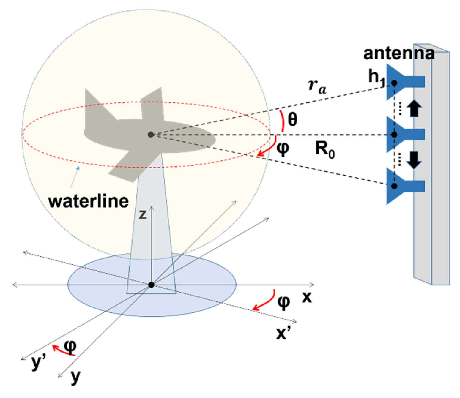
The setup for a 3D scan is illustrated in Fig. 1. A target was positioned on a turntable rotating at angle ϕ, and transmitter (Tx) and receiver (Rx) antennas were moved together along the vertical tower to collect scattering information at different heights (h). The Rx antenna received only co-polarized signals from the Tx antenna. Radio frequency (RF) data were obtained using the stepped-frequency continuous-wave method. Consider the target a set of independent point scatterers where the reflectivity was ρ(r). The backscattered electric field (u) measured by the Rx antenna is given by the following equation:

where r_a is the antenna position vector, f is the frequency, k is the wave number, G is the antenna gain, and V is the target volume [7]. In this case, G can be omitted for brevity. ρ(r) is depicted as a pixel in the radar image, and its size is inversely proportional to the scan length [14]. After collecting the backscattered field u, we can evaluate the individual point scatterers using the reverse form of Eq. (1):

where B is the frequency bandwidth [4, 6, 7, 9]. Here, the kernel function ( ∣r-ra∣2e-j2k∣r-ra∣) is the focusing operator that gives all the individual point scatterers of a target based on the NF data collected. If the target height is short, a 3D full scan can be replaced by a 2D azimuth scan in the waterline direction (i.e., θ = 0). The focusing algorithm for the 2D scan can be written as follows:

where r_ϕ is the antenna position vector when θ = 0. The target scattering pattern S and RCS are then calculated using a set of scattering points ρ(r):

where r̂ is the directional vector of antenna (r_a) and σ is the RCS.

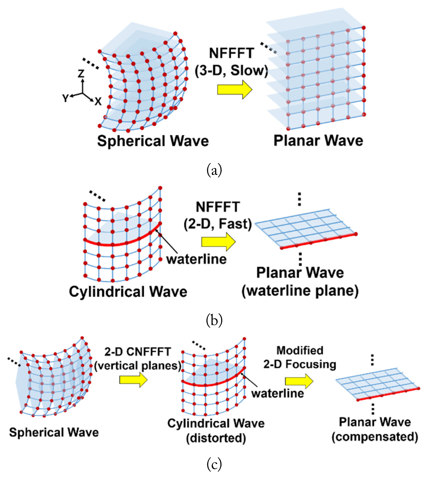
According to Sensani et al. [9], direct integration of a focusing operator is more accurate than any other fast-Fourier-transform-based imaging process technique. However, for 3D cases, this operation requires an enormous computational load, which causes too much time delay (Fig. 2(a)).

We should note that the 2D operation is valid only if the received field satisfies the FF criterion in the vertical direction (i.e., a cylindrical waveform), as shown in Fig. 2(b). To satisfy this condition, the first step of the subdimensional conversion is to alter the collected spherical waveform to form a cylindrical one using the CNFFFT method. In other words, every r-θ subplane is converted to the r-z subplane, expressed as follows:

where M is the total number of r-z subplanes, S_cyl is the converted cylindrical scattering pattern for a single r-z subplane, Hq(1) is the Hankel function of the first kind, U is the derivative of the NF backscattered electric field with regard to k, N = kD + 10 is the monostatic spherical-mode cutoff of the target, and d is the minimum diameter of a sphere that includes the whole size of the target and has the same center as the turntable [7]. However, the cylindrical waveform generated by Eq. (6) is slightly distorted due to the inherent approximation term of CNFFFT itself.

Specifically, the aforementioned error becomes more severe as the ratio of the target dimension to the measurement distance increases. However, we resolved this error by adding the term ∣r-ra∣/∣ra∣ in the focusing operator. This was done because this term can replace the approximated distance ( 1∣ra∣) for each point scatterer with a precise one ( 1∣ra-r∣) individually. Therefore, our final model for the focusing operation is written as follows:

where the term e-j2krϕ[(r-rϕ)·rϕ^]2 is used to transform the scattering pattern (S_cyl) into the field at antenna position r_ϕ.

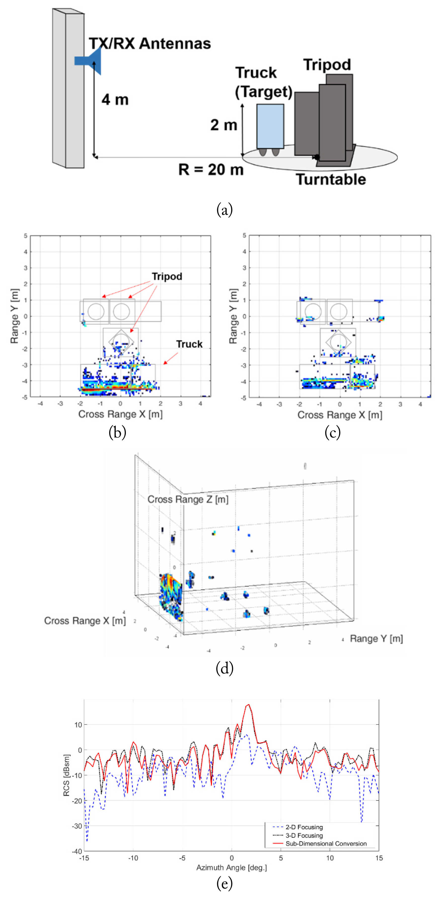
First, we measured the NF of a truck sample with the dimensions 3.8 m (L) × 1.5 m (W) × 2.0 m (H) (Fig. 3(a)). The measurement distance was 20 m. The central frequency was 3.2 GHz, with a 2 GHz bandwidth (2.2–4.2 GHz, with 1,051 samples), and the azimuth angle was from −17.5° to 17.5°, with 121 samples. The center height of the Tx and Rx antennas was 4 m, and the vertical scan length was 6 m, with 0.1 m steps. The tripod was covered with radar-absorbing material. We applied subdimensional conversion to extrapolate the FF radar image and RCS pattern. For comparison, we also used direct integration of a focusing operator (focusing operation).

Fig. 3 shows a set of constructed radar images of the truck sample. The major component contributing to the backscattered field was the side surface of the truck, which was equivalent to a rectangular metallic plate. At this 20 m range, the backscattered field in the vertical direction could not meet the standard FF criterion.

where R, D, and λ are the measurement distance, target dimension, and wavelength, respectively. Thus, a 2D focusing operation with a 2D scan at the antenna center height was insufficient to create a reliable FF radar image (Fig. 3(c)). Accordingly, the RCS peak attributed to the normal reflection from the side surface does not appear in Fig. 3(e) (blue-dotted line). On the other hand, very intense reflection from this surface was observed in the image constructed through subdimensional conversion (Fig. 3(b)). This is because the NF received in the vertical direction was converted to FF by CNFFFT. This surface was also clearly constructed in a 3D image generated by the 3D focusing operation (Fig. 3(d)). The resulting RCS patterns were almost identical in both cases. However, as shown in Table 1, the processing speed for the subdimensional conversion was much faster than that for the 3D focusing operation. The 3D focusing algorithm and subdimensional conversion can also be compared in terms of analytical complexity. The complexity of Eq. (2) is O(lmn), but the complexity of Eq. (9) is O(n)+O(lm), where l is the number of frequency samples, m is the number of azimuth angle samples, and n is the number of vertical samples. In Eq. (9), regardless of r and ϕ, it is first computed for θ in Eq. (6).

Furthermore, subdimensional conversion enabled us to reduce the vertical scan length without sacrificing accuracy. According to Eq. (11), cross-range resolution and vertical scan length are directly related to each other.

where ρ_CR–V is the vertical cross-range resolution, λ is the wavelength, R₀ is the distance of the target from the antenna, and L is the vertical scan length [9]. In particular, for low-frequency or long-range measurements, it is hard to secure a fine vertical cross-range resolution (ρ_CR–V) due to the physical restriction of long-range vertical scanning. Thus, low-quality radar images are created, which are not appropriate for the accurate extraction of an RCS. However, with the subdimensional conversion method, the CNFFFT method converts to the FF in the vertical direction. Because CNFFFT does not produce an intermediate-constructed radar image and does not convert to FF from an explicit radar image, the size of ρ_CR–V is of no concern for the extraction of an accurate RCS. This advantage allows for the shortening of the vertical scanning length and time.

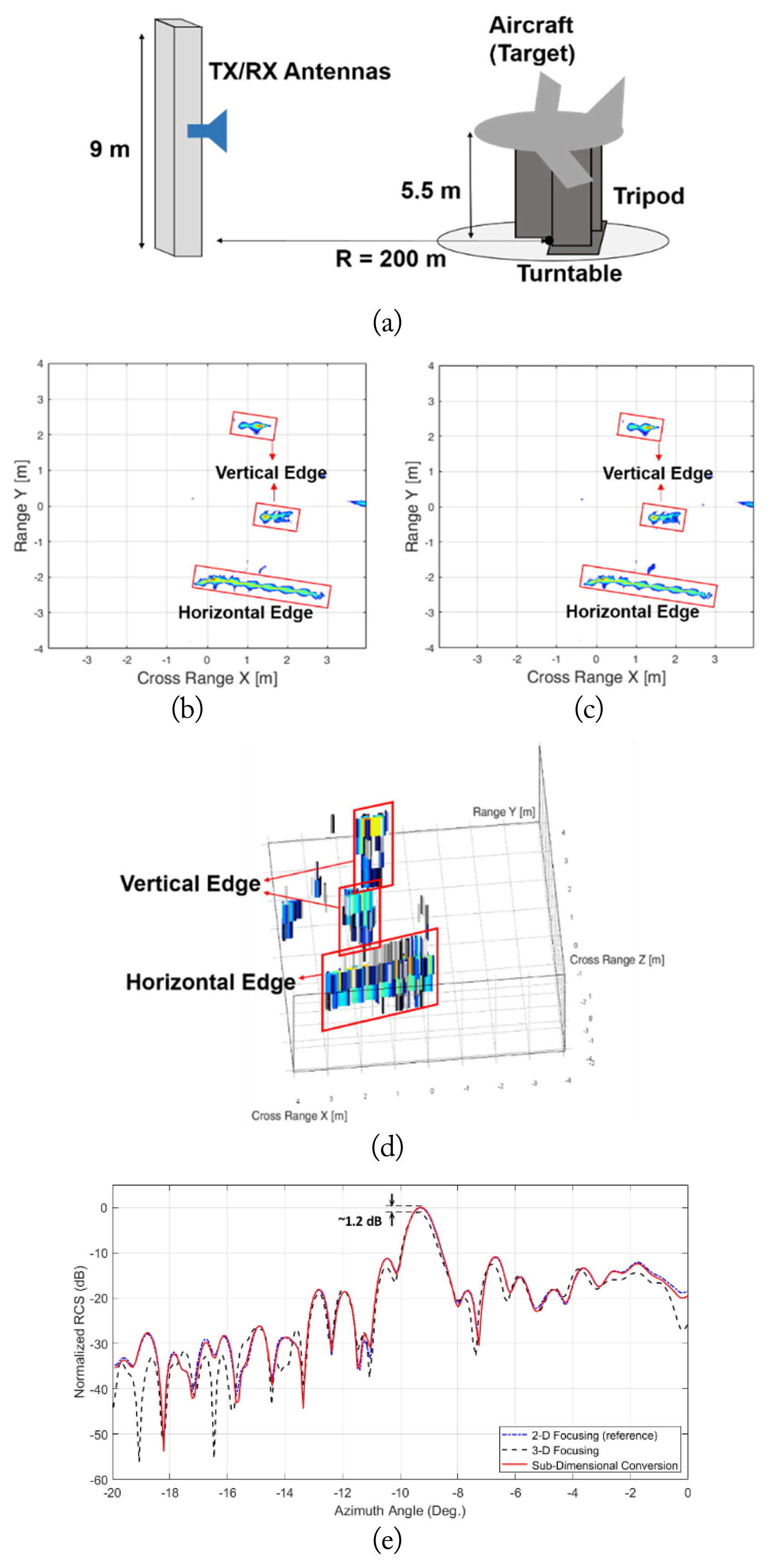
The aforementioned speculation was demonstrated using an NF scan of the aircraft model with the dimensions 10.5 m (L) × 7 m (W) × 2.3 m (H) (Fig. 4(a)). Here, the measurement distance was 200 m, and the frequency was 3.2 GHz, with a 2 GHz bandwidth (2.2–4.2 GHz, with 1,401 samples). The horizontal and vertical edges were aligned in the azimuth direction, and the azimuth scan angle included this direction. The vertical scan range was 9 m, with 0.3 m steps. The vertical height of the aircraft model was 2.3 m, and, according to Eq. (10), the minimum length needed to guarantee that FF will be in the vertical direction is ~112 m, which is even shorter than our measured distance (200 m). Therefore, as references, a 2D FF radar image and an RCS pattern were extracted using a 2D focusing operation with 2D scanning.

Fig. 4(d) shows a filtered 3D radar image of the aircraft mock-up created using a 3D focusing operation. Except for the horizontal and vertical edges, all the other scattering points were filtered by the image-gating function. Because ρ_CR–V was too large (~1.04 m), the image quality was severely degraded in the vertical direction; point scatterers composed of the horizontal and vertical edges were spread by an over 3 m length in the vertical direction. Hence, the distorted image resulted in an inaccurate RCS pattern (black-dotted line in Fig. 4(e)) that deviated from that extracted by the 2D focusing operation (reference, blue-dotted line in Fig. 4(e)). This result suggests that a longer vertical scan is needed to obtain more accurate RCS patterns when a 3D focusing operation is used. In contrast, a 2D image constructed through subdimensional conversion (Fig. 4(b)) is almost identical to that constructed by the 2D focusing operation (Fig. 4(c)). Therefore, excellent concurrence is identified in the RCS patterns in Fig. 4(e) (red line vs. blue-dotted line), indicating that the 9 m vertical scan length is sufficient for extracting accurate images and RCS patterns. We expect that the vertical scan length can still be further reduced without compromising the determined accuracy level of the RCS.

In this paper, a subdimensional hybrid conversion method is proposed as a relevant 3D IB NFFFT algorithm. It has shown better efficiency in RCS extraction than direct integration of a 3D focusing operator. Moreover, unlike with other IB NFFFT techniques, we found that its conversion accuracy was maintained even if the vertical scan length was relatively short. This will be very useful for reducing the total scanning time.