Analysis Method for Determining Optimal Synthetic Aperture Time Using Estimated Range and Doppler Cone Angle at the Center of Synthetic Aperture Length

Article information

J. Electromagn. Eng. Sci. 2023;23(3):205-211

doi : https://doi.org/10.26866/jees.2023.3.r.160

Advanced Defense Science & Technology Research Institute, Agency for Defense Development, Daejeon, Korea

^*Corresponding Author: Min-Ji Kim (e-mail: hami3426@add.re.kr)

Received 2022 July 26; Revised 2022 November 19; Accepted 2023 January 19.

Abstract

Synthetic aperture time (SAT) is a crucial component for acquiring high-quality synthetic aperture radar images with an excellent target cross-range resolution. SAT is analyzed using the range and Doppler cone angle at the center of the synthetic aperture length (SAL). However, in a real flight mission setting, only the range and Doppler cone angle at the SAL’s starting point are determined. Therefore, we present a method for estimating the range and Doppler cone angle at the center of the SAL to calculate an accurate SAT that is suitable for the spatial resolution of the assigned mission. We performed an iterative analysis of SAT at the range and Doppler cone angle at the starting point of the SAL (original SAT) and at the center of the SAL (proposed SAT). Consequently, the proposed SAT decreased by 0.69%–16.14% compared to the original SAT at a resolution of 0.1–3.0 m.

Keywords: Synthetic Aperture Length (SAL); Synthetic Aperture Radar (SAR); Synthetic Aperture Time (SAT)

I. Introduction

Synthetic aperture radar (SAR) is a powerful remote sensing technology that uses the signal it receives from the target region to create an image [1–8]. Parameters such as spatial resolution, noise equivalent sigma zero, peak sidelobe ratio, and integrated sidelobe ratio [9, 10] are used to evaluate image quality. Numerous studies have been conducted to improve the spatial resolution of SAR images [11–16]. Spatial resolution consists of two components: range and cross-range resolution. Range resolution is enhanced by transmitting a pulse with a wide bandwidth [11].

Additionally, high cross-range resolution is achieved by synthesizing the collected data while the SAR sensor is in motion. Cross-range resolution can be improved as the time and length of synthesis increase; these factors are referred to as the synthetic aperture time (SAT) and synthetic aperture length (SAL), respectively. However, the time for image formation also increases at the same rate. Therefore, it is necessary to identify optimal SAT and SAL values that can satisfy the target image cross-range resolution.

SAT is analyzed based on the wavelength, slant range between the platform and the ground target, Doppler cone angle between the platform velocity vector and the line of sight to the ground target, cross-range resolution, and platform velocity [17].

The slant range has a nominal value [17], which is usually the distance between the platform and the ground target when the platform is positioned at the center of the SAL. The Doppler cone angle is the angle between the platform’s velocity vector and the radar line of sight to the ground target at the center of the SAL. However, when starting signal synthesis in a real flight mission setting, only the range and Doppler cone angle at the starting point of the SAL can be determined, while the range and Doppler cone angle at the center of SAL remain unknown. Therefore, it is necessary to estimate the range and Doppler cone angle at the center of the SAL to calculate an accurate SAT that is suitable for the resolution of the assigned mission.

Earlier studies [18, 19] did not consider the actual mission environment and instead used the slant range between the center of the SAL and the target as an arbitrary constant value to solve the unknown parameters in the SAR geometry. In other studies [11, 20, 21], when performing an SAR simulation, the slant range from the center of the SAL was assumed to be a constant value and that from the SAL’s starting point, which is known in the current mission environment, was not considered. In this paper, we present a method for estimating the range and Doppler cone angle at the center of the SAL and the optimal SAT.

This paper consists of the following sections. The range and Doppler cone angle estimation method is discussed in Section II. In Section III, we analyze and compare the SAT derived by using the initial range and Doppler cone angle (original SAT) and the SAT derived using the estimated range and Doppler cone angle (proposed SAT) with resolutions of 0.1 m, 0.3 m, 0.5 m, 1.0 m, and 3.0 m. Additionally, we simulate the impulse response function (IRF) of a point target to explain the proposed method and review the results. Section IV provides a brief conclusion to the overall study.

II. Estimation Method of the Range and Doppler Cone Angle at the Center of the SAL

1. SAR Geometry

Fig. 1 illustrates the SAR geometry. When the platform moves through the flight path to synthesize the image with the target cross-range resolution, SAT is analyzed as follows [17]:

Fig. 1

SAR geometry.

(1) SAT=λRKa2vρasin(θ),

where λ is the wavelength, R is the distance between the platform and the ground target, K_a is the generalized mainlobe-broadening factor introduced by aperture weighting, v is platform velocity, v is the cross-range resolution, and θ is the Doppler cone angle between the platform’s velocity vector and the radar’s line of sight to the ground target. In Fig. 1, the SAL is the aperture length used to synthesize the signal and is determined by the following equation:

(2) SAL=SAT×v,

where SAT is the synthetic aperture time and v is the platform velocity.

2. Estimation Method

Fig. 2 depicts the flow diagram for estimating the range (R_c) and Doppler cone angle (θ_c) at the center of the SAL. The initial slant range (R_s), initial angle between the platform velocity vector and the line of sight to the ground target (θ_s) in Fig. 1, wavelength (λ), platform velocity (v), and cross-range resolution (ρ_as) at the starting point of the SAL were used to determine SATs and SALs. From the acquired SALs, we determined the slant range at the center of the SAL (R_c), slant range at the end of the SAL (R_e), and angle (θ_c), as depicted in Fig. 1.

Fig. 2

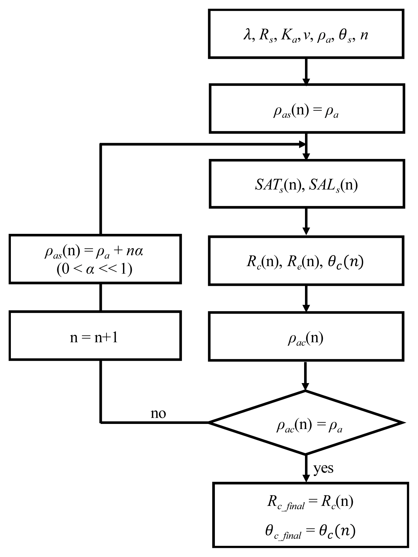
Flow diagram to explain the estimation method of the range (R_c) and the Doppler cone angle (θ_c) at the center of the SAL.

(3) Rc(n)=Rs2+(SALs(n)2)2-2Rs(SALs(n)2)cos(θs),

(4) Re(n)=Rs2+(SALs(n))2-2Rs(SALs(n))cos(θs),

(5) θc(n)=cos-1 ((Rc(n)) 2+(SALs(n)2)2-(Re(n))2Rc(n)SALs(n)),

where n is the number of trials. By calculating R_c(n) and θ_c(n), we can confirm the nth cross-range resolution (ρ_ac(n)) at the center of the SAL from the following:

(6) ρac(n)=λRc(n)Ka2vSATs(n)sin(θc(n)),

where λ is the wavelength, v is platform velocity, and SAT_s(n) is the n^th synthetic aperture time. The computed cross-range resolution (ρ_ac(n)) was then compared to the target cross-range resolution (ρ_a). As stated in Eq. (7)n is increased by 1 and the cross-range resolution at the starting point of the SAL is modified if the two values do not match:

(7) ρas(n)=ρa+nα,

where ρ_a is the target cross-range resolution, n is the number of trials and a natural number, and α is a value greater than 0 and considerably less than 1.

We then repeatedly calculated SAT_s(n), SAL_s(n), R_c(n), R_e(n), θ_c(n), and ρ_ac(n) using the previously determined cross-range resolution (ρ_as), R_s, θ_s in Fig. 1, λ, and v. If the value of ρ_ac(n) is equal to the value of ρ_a, then R_c(n) and θ_c(n) are the final estimated range and Doppler cone angle at the center of the SAL, respectively. At this time, the last SAT that satisfies the target cross-range resolution at the center of the SAL is SAT_s(n).

III. Results and Discussion

1. SAT Analysis Results

SAT analysis is performed to compare the SAT by initial range and Doppler cone angle at the starting point of the SAL and SAT by the estimated range and Doppler cone angle at the center of the SAL. SAT by initial range and Doppler cone angle is referred to as the original SAT, and SAT by estimated range and Doppler cone angle is referred to as the proposed SAT in this chapter, for convenience.

Table 1 illustrates the prerequisites for SAT analysis. The cross-range resolutions of the target are 0.1, 0.3, 0.5, 1.0, and 3.0 m. The height of the platform is 10 km, and its velocity is 100 m/s. The initial slant range (R_s) is 80 km. The frequency utilized is in the X-band range. Fig. 3 depicts an analysis of the results of the original and proposed SATs at a resolution of 0.1–3.0 m. K_a is assumed to be a Taylor aperture weighting (−35 dB, nbar = 5) for assessing the SAT.

Table 1

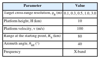
Preconditions for SAT analysis

Fig. 3

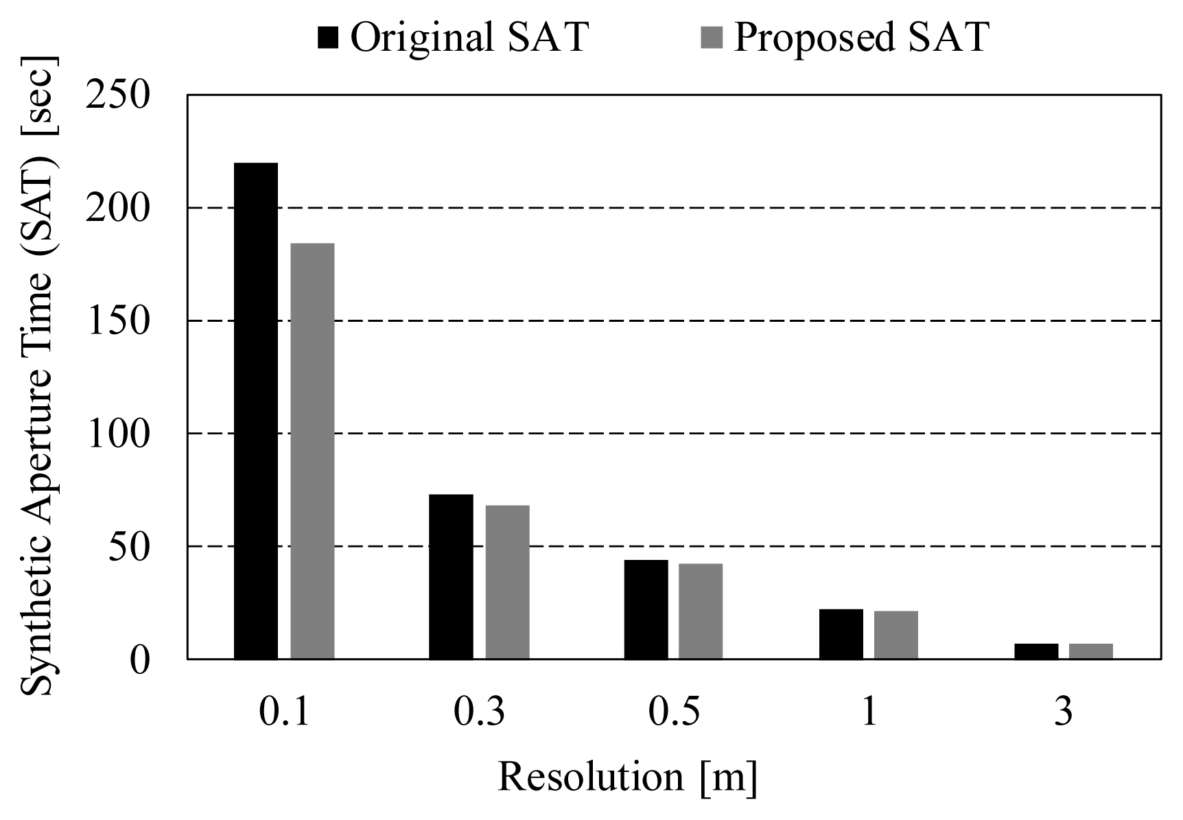
Analysis results of original and proposed SAT.

The original SAT was calculated to be 219.22, 73.07, 43.84, 21.92, and 7.31 seconds for the resolutions of 0.1, 0.3, 0.5, 1.0, and 3.0 m, respectively. The proposed SAT values are 183.83, 68.46, 42.12, 21.48, and 7.26 seconds for the resolutions of 0.1, 0.3, 0.5, 1.0, and 3.0 m, respectively. Based on these results, we could confirm that the proposed SAT was 0.69%–16.14% less than the original SAT. Additionally, we found that the proposed SAT decreased at a higher rate than the original SAT as the resolution enhanced.

2. Simulation Results

We performed an IRF simulation for a point target on the ground to clarify the estimation method. The geometry of the point target is depicted in Fig. 1. We used the polar format algorithm (PFA) for the image formation of the point target. The PFA is the most suitable imaging algorithm for high-resolution squinted spotlight SAR [22].

Fig. 4 illustrates the flow diagram for simulating a point target on the ground. The blue box in Fig. 4 depicts the PFA. The prerequisites for IRF simulation are summarized in Table 2. The pulse numbers of the waveform are derived from the original and proposed SATs, respectively, in Table 2.

Fig. 4

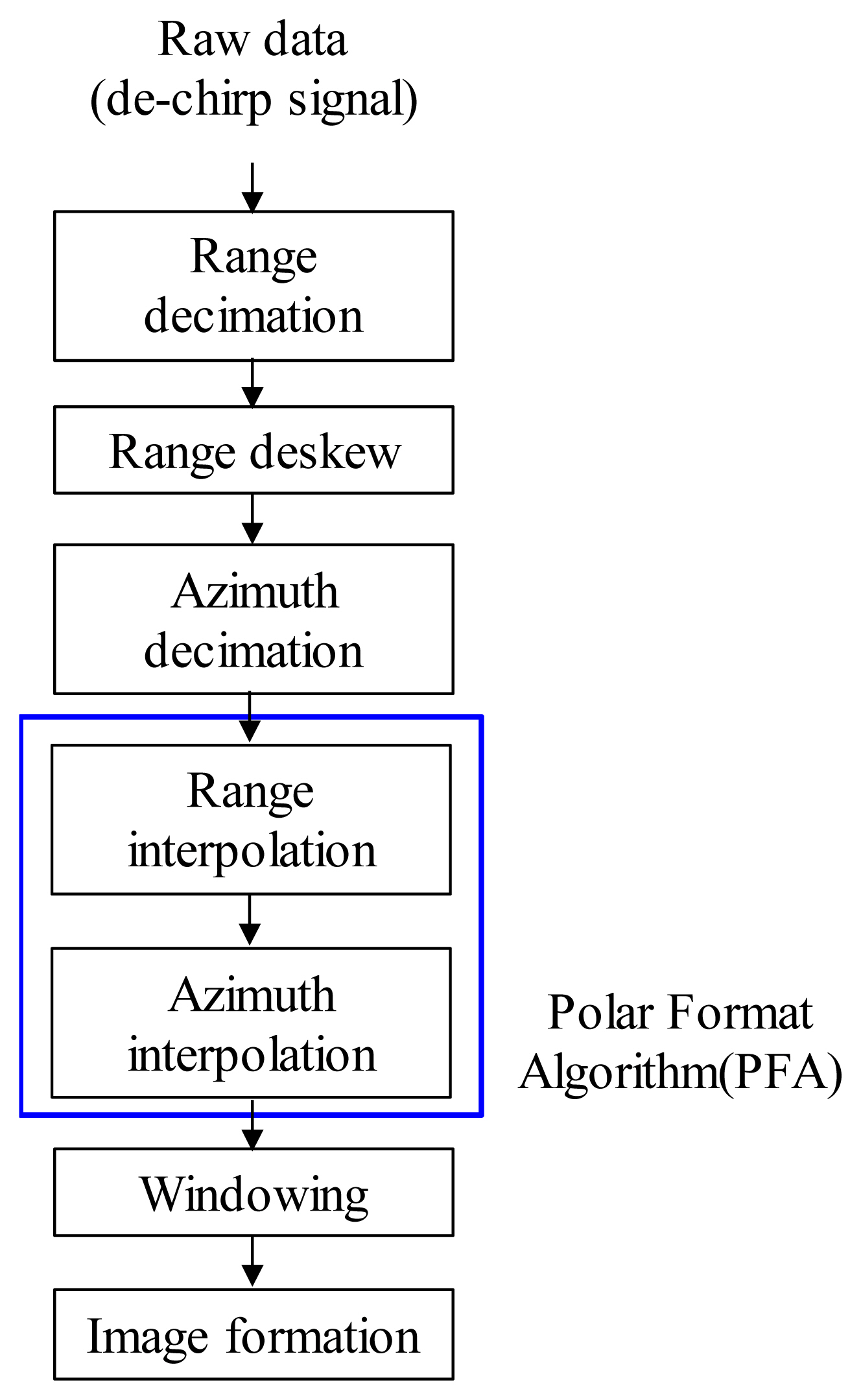
Flow diagram to simulate a point target on the ground.

Table 2

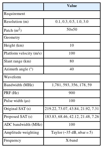
Preconditions for impulse response function simulation

Figs. 5 and 6 depict the IRF results simulated from the waveform derived by the original and proposed SATs, respectively. Based on these simulation results, we could confirm that although the proposed SAT was 0.69%–16.14% less than the original SAT, the cross-range resolutions of the images formatted by the proposed SAT were 0.10, 0.30, 0.49, 0.99, and 2.99 m, which satisfied the target cross-range resolutions of 0.1, 0.3, 0.5, 1.0, and 3.0 m.

Fig. 5

IRF results simulated from the waveform derived using the original SAT for target cross-range resolutions of (a) 0.1 m, (b) 0.3 m, (c) 0.5 m, (d) 1.0 m, and (e) 3.0 m.

Fig. 6

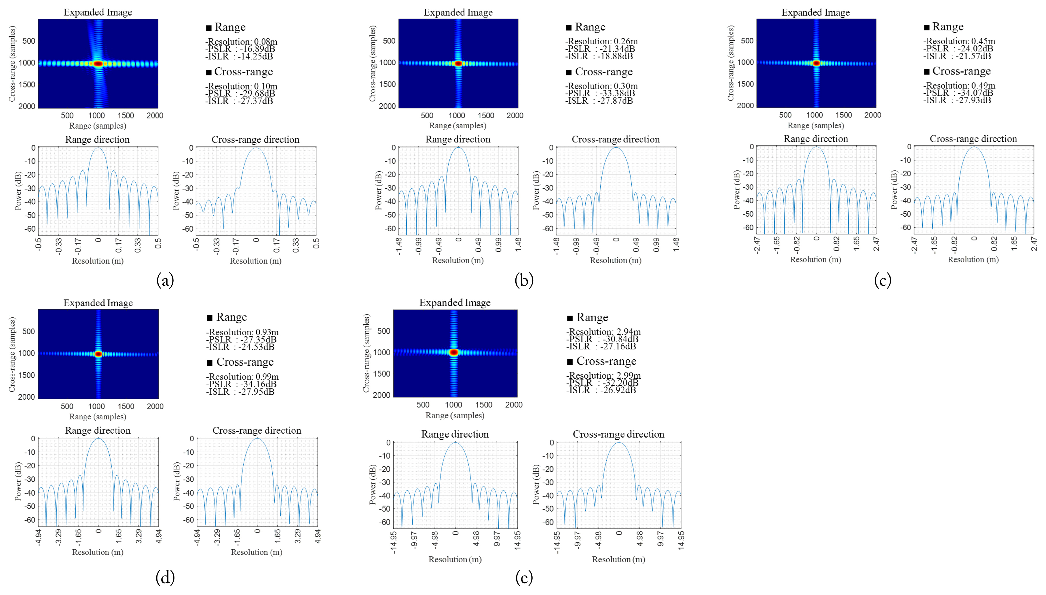
IRF results simulated from the waveform derived using the proposed SAT for target cross-range resolutions of (a) 0.1 m, (b) 0.3 m, (c) 0.5 m, (d) 1.0 m, and (e) 3.0 m.

3. Discussion

This paper proposed a method to estimate the slant range and Doppler cone angle at the center of the SAL to determine an accurate SAT that is suitable for the resolution of an assigned mission. To verify the proposed estimation method, we analyzed the SAT in a cross-range resolution of 0.1–3.0 m and performed an IRF simulation of a point target using the original SAT and proposed SAT.

From this, we established that although the proposed SAT, at 0.69%–16.14%, was less than the original SAT, the cross-range resolution of the formatted image matched the desired cross-range resolution of 0.1–3.0 m. Flight time can be reduced by utilizing the proposed estimation method during an actual mission.

However, additional time is required for performing the iterative method. We confirmed that about 0.08 seconds is additionally required for cross-range resolution of 0.1 m and α of 0.00001 under the conditions outlined in Table 2 (MATLAB tool). The estimation time of 0.08 seconds can be regarded as insignificant compared with the original and proposed SAT times of 219.22 and 183.83 seconds, respectively, for a cross-range resolution of 0.1 m. However, as the value of α increases, the estimation time increases; thus, it is necessary to select an appropriate α. In this study, the value was selected as 0.00001.

IV. Conclusion

We presented a method of analysis for optimal SAT by estimating the range and Doppler cone angle at the center of the SAL. To verify the estimation method, we analyzed the SAT in cross-range resolutions of 0.1, 0.3, 0.5, 1.0, and 3.0 m and performed IRF simulations of the point target using both the original and proposed SATs. The SAT analysis revealed that the proposed SAT decreased by 0.69%–16.14%, compared to the original SAT, for a target cross-range resolution of 0.1–3.0 m. We confirmed that although the proposed SAT was 0.69%–16.14% less than the original SAT, the cross-range resolution of the image formatted by the proposed SAT matched the target cross-range resolution of 0.1–3.0 m.

The proposed range and Doppler cone angle estimation method in this paper has applications in determining the optimal flight time for SAR images with target cross-range resolution.

Acknowledgments

This work was supported by the Agency for Defense Development by the Korean Government.

References

1. Bovenga F.. Special issue: synthetic aperture radar (SAR) techniques and applications. Sensors 20(7)article no. 1851. 2020;https://doi.org/10.3390/s20071851.

2. Villano M., Krieger G., Moreira A.. New insights into ambiguities in quad-pol SAR. IEEE Transactions on Geoscience and Remote Sensing 55(6):3287–3308. 2017;

3. Chen H., Shi Z.. A spatial-temporal attention-based method and a new dataset for remote sensing image change detection. Remote Sensing 12(10)article no. 1662. 2020;https://doi.org/10.3390/rs12101662.

4. Gao Y., Gao F., Dong J., Wang S.. Change detection from synthetic aperture radar images based on channel weighting-based deep cascade network. IEEE Journal of Selected Topics in Applied Earth Observations and Remote Sensing 12(11):4517–4529. 2019;

5. Zhang X., Liu G., Zhang C., Atkinson P. M., Tan X., Jian X., Zhou X., Li Y.. Two-phase object-based deep learning for multi-temporal SAR image change detection. Remote Sensing 12(3)article no. 548. 2020;https://doi.org/10.3390/rs12030548.

6. Giustarini L., Hostache R., Matgen P., Schumann G. J. P., Bates P. D., Mason D. C.. A change detection approach to flood mapping in urban areas using TerraSAR-X. IEEE Transactions on Geoscience and Remote Sensing 51(4):2417–2430. 2013;

7. Lee M. J., Kang M. S., Ryu B. H., Lee S. J., Lim B. G., Oh T. B., Kim K. T.. Improved moving target detector using sequential combination of DPCA and ATI. The Journal of Engineering 2019(21):7834–7837. 2019;

8. Kang M. S., Kim K. T.. Compressive sensing based SAR imaging and autofocus using improved Tikhonov regularization. IEEE Sensors Journal 19(14):5529–5540. 2019;

9. Kang M. S., Won Y. J., Lim B. G., Kim K. T.. Study on spaceborne SAR system performance improvements using antenna pattern resynthesis in presence of element failure. The Journal of Korean Institute of Electromagnetic Engineering and Science 29(8):624–631. 2018;

10. Riche V., Meric S., Baudais J. Y., Pottier E.. Investigations on OFDM signal for range ambiguity suppression in SAR configuration. IEEE Transactions on Geoscience and Remote Sensing 52(7):4194–4197. 2014;

11. Lim S., Choi I., Jeong T.. Compensation method for a wideband signal’s squint problem of an AESA SAR system using a cross-range-variant antenna gain equalizer. IEEE Sensors Journal 19(8):2937–2945. 2019;

12. Zhai W., Zhang Y.. A stepped frequency chirp scaling algorithm for high resolution SAR imaging. In : Proceedings of 2011 3rd International Asia-Pacific Conference on Synthetic Aperture Radar (APSAR). Seoul, South Korea; 2011; p. 1–4.

13. Shibo X., Jialong G., Bocai W.. Research on high resolution SAR based on frequency-stepped chirps. In : Proceedings of 2009 2nd Asian-Pacific Conference on Synthetic Aperture Radar. Xi’an, China; 2009; p. 103–107.

14. Zhai W., Zhang Y.. Application of super-SVA to stepped-chirp radar imaging with frequency band gaps between subchirps. Progress in Electromagnetics Research B 30:71–82. 2011;

15. Deng Y., Zheng H., Wang R., Feng J., Liu Y.. Internal calibration for stepped-frequency chirp SAR imaging. IEEE Geoscience and Remote Sensing Letters 8(6):1105–1109. 2011;

16. Zeng L., Liang Y., Xing M., Huai Y., Li Z.. A novel motion compensation approach for airborne spotlight SAR of high-resolution and high-squint mode. IEEE Geoscience and Remote Sensing Letters 13(3):429–433. 2016;

17. Carrara W. G., Goodman R. S., Majewski R. M.. Soptlight Synthetic Aperture Radar: Signal Processing Algorithms Boston, MA: Artech House; 1995.

18. Guo Z., Fu Z., Chang J., Wu L., Li N.. A novel high-squint spotlight SAR raw data simulation scheme in 2-D frequency domain. Remote Sensing 14(3)article no. 651. 2022;https://doi.org/10.3390/rs14030651.

19. Xu W., Huang P., Deng Y.. Efficient sliding spotlight SAR raw signal simulation of extended scenes. EURASIP Journal on Advances in Signal Processing 2011article no. 52. 2011;https://doi.org/10.1186/1687-6180-2011-52.

20. Bu L., Zhao S., Zhang G., Song R.. Simulations of spotlight synthetic aperture radar super-resolution algorithm. Journal of the Indian Society of Remote Sensing 50:493–505. 2022;https://doi.org/10.1007/s12524-021-01469-5.

21. Lee H., Kim K. W.. An integrated raw data simulator for airborne spotlight ECCM SAR. Remote Sensing 14(16)article no. 3897. 2022;https://doi.org/10.3390/rs14163897.

22. Nie X., Shen S., Yu H., Liu Y., Zhuang L., Lei W.. A wide-field SAR polar format algorithm based on quadtree sub-image segmentation. In : Proceedings of 2018 IEEE International Geoscience and Remote Sensing Symposium (IGARSS). Valencia, Spain; 2018; p. 9355–9358.

Biography

Min-Ji Kim received her B.S. degree in Electrical Engineering and Computer Science from Kyung-Pook National University, Daegu, South Korea, in 2009 and her M.S. and Ph.D. degrees in Bio and Brain Engineering from Korea Advanced Institute of Science and Technology (KAIST), Daejeon, South Korea, in 2011 and 2016, respectively. Since March 2016, she has been a Senior Researcher with the Agency for Defense Development (ADD), Daejeon, South Korea. Her current research interests include synthetic aperture radar and airborne radar systems and signal processing.

Sangho Lim received his B.S. degree from Chung-Ang University, Seoul, South Korea, in 2006 and his Master’s and Ph.D. degrees from the Korea Advanced Institute of Science and Technology (KAIST), Daejeon, South Korea, in 2008 and 2011 respectively, all in electrical engineering. From 2011 to 2016, he was with Samsung Electronics Co., Ltd., Suwon, South Korea, as a Senior RF and Antenna Engineer, where he was involved in extensive research and development tasks for wireless applications including 5G communications, wireless power transfer, and mm-wave wireless solutions. Since 2016, he has been with Agency for Defense Development (ADD), Daejeon, South Korea. He is currently a Principal Researcher with Radar & EW Technology Center at ADD. He has authored or co-authored over 35 articles in peer-reviewed journals and conference papers. He has over 40 patent inventions. His current research interests include synthetic aperture radar and space situational awareness radar.

Dong-Cho Shin received his Master’s degree in Computer Science from Choongnam National University, South Korea, in 1995. Since February 1997, he has been with the Agency for Defense and Development, South Korea, where he is currently a Chief-Principal Researcher. His research interests include airborne air-to-ground radar systems.

Article information Continued

This is an Open-Access article distributed under the terms of the Creative Commons Attribution Non-Commercial License (http://creativecommons.org/licenses/by-nc/4.0) which permits unrestricted non-commercial use, distribution, and reproduction in any medium, provided the original work is properly cited.

Funded by : Agency for Defense Development by the Korean Government

Funding : This work was supported by the Agency for Defense Development by the Korean Government.

Parameter	Value
Target cross-range resolution, ρ_a (m)	0.1, 0.3, 0.5, 1.0, 3.0
Platform height, H (km)	10
Platform velocity, v (m/s)	100
Range at the starting point, R_s (km)	80
Azimuth angle, θ_az (°)	40
Frequency	X-band

	Value
Requirement
Resolution (m)	0.1, 0.3, 0.5, 1.0, 3.0
Patch (m²)	50×50
Geometry
Height (km)	10
Platform velocity (m/s)	100
Slant range (km)	80
Azimuth angle (°)	40
Waveform
Bandwidth (MHz)	1,781, 593, 356, 178, 59
PRF (Hz)	900
Pulse width (μs)	100
Original SAT (s)	219.22, 73.07, 43.84, 21.92, 7.31
Proposed SAT (s)	183.83, 68.46, 42.12, 21.48, 7.26
ADC bandwidth (MHz)	100
Amplitude weighting	Taylor (−35 dB, nbar = 5)
Frequency	X-band