Using the CLEAN Method in Three-Dimensional Polarimetric ISAR Imaging Based on Volumetric Scattering Points
Article information

Abstract
We developed a new technique for generating three-dimensional monostatic inverse synthetic aperture radar (ISAR) images using various types of polarimetric information on targets. To remove clutter around a target, we adopted the CLEAN method, in which only the main signals were reconstructed using an iterative algorithm. We conducted a simulation as follows: electric field data that were subjected to polarimetric scattering were obtained for the target using a full-wave electromagnetic analysis simulator. The linear polarization data of a 2 × 2 matrix were compressed into the linear to circular polarization data of a 2 × 1 matrix using the Jones vector based on circular polarization. On the grounds of the post-processed data, inverse Fourier transform was carried out to map scattering points to the spatial domain, after which the CLEAN method was used to retain only the primary scattering points.
I. INTRODUCTION
Radar imaging is used for automatic target recognition (ATR) and automatic target classification (ATC) because it can indicate the shape and structural characteristics of a target using scattered wave data. In particular, inverse synthetic aperture radar (ISAR) imaging generates an image by synthesizing scattered wave signals from the various look angles of a target using a fixed radar system [1].
Three-dimensional (3D) ISAR imaging more accurately represents the distribution of a target’s scattering points than its two-dimensional (2D) counterpart, as the former can render such points in three coordinate axes and is extensively used in ATR and ATC [1, 2]. A 3D ISAR imaging also involves adding a dimension to an ISAR image projected onto an image projection plane (IPP). Such images have been generated through various methods [2], among which some general approaches are the adoption of a single monostatic radar and a bistatic ISAR and the multiple-input and multiple-output ISAR method that employs two or more radars [3].
In the abovementioned radar systems, 3D ISAR imaging can be implemented in different ways. Examples include ISAR movie imaging, 3D turntable ISAR imaging, and interferometric ISAR (In-ISAR) imaging, which involves the formation of a 3D image using the interferometric phases of different antennas [3].
In this research, we performed 3D ISAR imaging using a monostatic radar that directly collects backscattered data in the radar line-of-sight (RLOS) direction and two Doppler (or cross-range) directions when a target rotates around the center of gravity [1]. The process then displays scattering points in the spatial domain [1]. This method is inexpensive in that it requires only one radar and entails an observation time shorter than that necessary in In-ISAR imaging.
In a radar system, the polarization of an electromagnetic wave is an important parameter that facilitates the derivation of various scattering data on a target [4]. Data subjected to horizontal-to-horizontal (HH), horizontal-to-vertical (HV), vertical-to-horizontal (VH), and vertical-to-vertical (VV) polarization are collected based on linear polarization and are generally used in a polarimetric radar system; these scattered wave signals are employed in analyzing the scattering information of a target [5–7]. In particular, an SAR system is adopted in scientific tasks, such as examining a wide range of soil characteristics using electric field data subjected to polarimetric scattering [4].
Information on the scattered wave signals of a target can differ according to polarization characteristics, and such information can be applied to the ISAR field. Various methods, such as the coherent or incoherent decomposition entailed in analyzing polarization information through the separation of base regions, have been developed and explored. In the current work, we demonstrated an approach to generating ISAR images by compressing a scattering matrix composed of four sets of the linear polarization data used in a general radar system into a matrix with two sets of polarization data through base transformation using a Jones vector [6, 7].
The rest of the paper is organized as follows: Section II explains how a basic monostatic ISAR image is formed and discusses the theory behind the polarimetric scattering of wave signals. It also describes the CLEAN method and presents the 3D scattering points required to generate 3D ISAR images. Section III recounts the formation of 3D ISAR images via simulation, and Section IV concludes with recommendations for future work.
II. SIGNAL MODELING
1. Formation of 3D Monostatic ISAR Images
A 3D ISAR imaging involves mapping the scattering points of a target to a 3D Cartesian coordinate system in the RLOS direction and in two directions perpendicular to the RLOS as coordinate axes. Scattering points can be defined in the range domain using the frequency bandwidth, or they can be defined in two Doppler (or cross-range) domains using the scattered wave signals collected at the azimuth and elevation angles around a target. If the target is cooperative, backscattered data at different look angles can be easily collected. However, in the case of a non-cooperative target, its side-scattered wave signals can be obtained using data derived from observations of the target in various directions using several radars or the rotational motion of the target itself [1, 8].
It is easy to design scattered wave signals for targets such as ships because their rotational motion is defined. That is, a ship makes a small rotational motion because of the influence of sea weather. This dynamic movement, which depends on maritime conditions and ship specifications, has a constant periodicity and can be assumed to be a uniform rotational motion. Therefore, scattered wave data can be acquired from observation points at equal intervals in the azimuth and altitude ranges of a target during a given radar observation period [8]. In this case, the ISAR of Doppler shift and cross-range domains may be defined equivalently [1]. During the coherent processing interval of a radar system, scattered electric field data can be collected from observation points at equal intervals in the azimuth and altitude angles of a target.
Here, Es(k, φ, ψ) denotes the K scattered electric field at the ri position of a target, Ai is the complex amplitude value at the ri position, and k=2πf⁄c is the propagation constant, where f is the frequency of the incident wave, and c represents the velocity of light. In the equation, as well, φ is the azimuth angle, and ψ=π⁄2−θ is the value obtained by subtracting the elevation from 90°. If the bandwidth (BW), the total azimuth angle (Ω), and the total elevation angle (Ψ) are small, scattered wave signals can be expressed using Eq. (1).
Scattering points can be mapped to the range domain by applying inverse Fourier transform (IFT) to the electric field in the frequency domain. Similarly, when backscattered signals are obtained at equal intervals at the azimuth and elevation angles, assuming a small bandwidth and a small observation angle, the scattering points in the cross-range direction can be calculated by applying IFT in the direction perpendicular to the RLOS [1].
In Eq. (2), ℱ−1{·} is the IFT operator, ISAR3D(x, y, z) denotes denotes a 3D ISAR in which a scattered electric field is expressed in the spatial domain, and C0 = (2BW/c) × (2fcΩ/c) × (2fcΨ/c) is a constant resulting from IFT application. The RLOS direction is parallel to the x-axis, and the azimuth and elevation directions are represented as the y- and z-axes, respectively. As shown in Eq. (2), the sinc function appears as a result of IFT given the limited range of the actual frequency and look angle [1]. A 3D ISAR image is ascribed a color that corresponds to the magnitude at each coordinate of ISAR3D(x, y, z). Unlike 2D ISAR imaging, which displays images only in the IPP that covers the RLOS, 3D ISAR imaging expands the dimension in the direction perpendicular to the IPP, thereby forming scattering points in the Cartesian coordinate system [2, 3].
2. Fully Polarimetric Backscattered Data
It has different types of information depending on the polarization of scattered electric field data. The polarization characteristics of scattered waves can be expressed by two orthogonal Jones vectors, and a polarimetric ISAR system using linear polarization is expressed as follows [4, 5]:
where EI is the incident electric field, ES refers to the scattering electric field, and S stands for the scattering matrix in which each element is the complex scattering amplitude. Each element is a result expressed based on linear polarization unit vector uH =(1,0)T and uV =(0,1)T. SHH and SVV represent co-polarization, wherein incident and scattered wave signals have the same polarization, whereas SHV and SVH reflect cross-polarization, in which incident and scattered waves have different polarizations [4]. An equivalent expression can be obtained by transforming the linear basis into a circular basis [5, 6]:
where L denotes the left direction, R indicates the right direction, and the left term can be divided into [SHL, SVL]T based on the left circular basis and into [SHR, SVR]T based on the right circular basis. From a macro perspective, these two are equivalent and can be used arbitrarily. Finally, the fully polarimetric signal of K scattering points is as follows:
Where
Additionally, AHL and AVL denote the complex amplitudes of the scattered signal of the left circular basis [6, 7]. In this research, ISAR images were formed using scattered electric field data obtained via the fully polarimetric method. The backscattered signal of each polarization was mapped to the spatial domain as Eq. (2).
3. CLEAN Method
The CLEAN method is a signal reconstruction technique involving the extraction of only the high-value segments of data that constitute a signal. It compresses data and improves the signal-to-noise ratio (SNR) [1, 9–11].
In Eq. (6), ISARre(x, y, z) is a 3D ISAR image reconstructed via the CLEAN method, An is the complex amplitude of the nth scattering point, and h(x, y, z) refers to the point spread function (PSF) that is an equivalent model of the original signal at the scattering points. The use of the CLEAN method to sequentially extract L PSFs with high values among the total K scattering points is illustrated in Eq. (7):
Where
which R0 is the residual power of the original ISAR, and Rn is the residual power of the nth ISAR. That is, the n-1th residual power is equal to the nth residual power minus the highest amplitude of PSFs. With an iterative solution, L scattering points above threshold amplitude AL can be obtained. Fig. 1 shows the target’s high-resolution range profile (HRRP), derived using 204 equally spaced range samples in the RLOS direction. The ISAR image was reconstructed using the CLEAN method, through which we extracted only five scattering points with a value exceeding a given threshold with 35% of normalized amplitude.
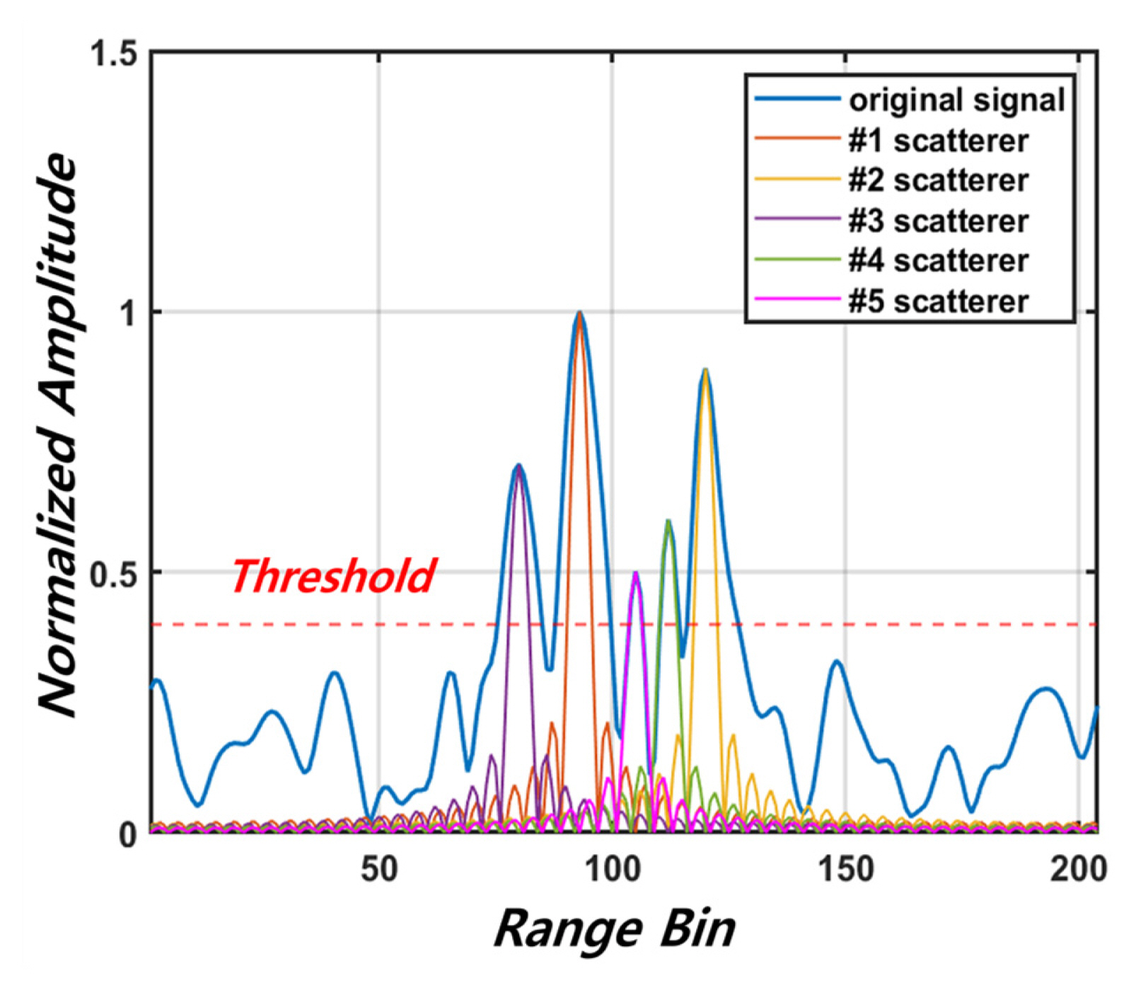
A 1D HRRP derived with the CLEAN method.
4. Volumetric Scattering Points
A scattered electric field in the spatial domain exists as a superposition of the signal as a sinc function at each coordinate point because of IFT. In the case of 3D ISAR imaging in a Cartesian coordinate system, the side lobes by the sinc function are listed in the direction parallel to the coordinate axis (Fig. 2) given that IFT was applied to the direction of each coordinate axis [9, 10, 12, 13]. Therefore, the volumetric scattering point defined by the PSF fundamentally uses the sinc function term of Eq. (5).
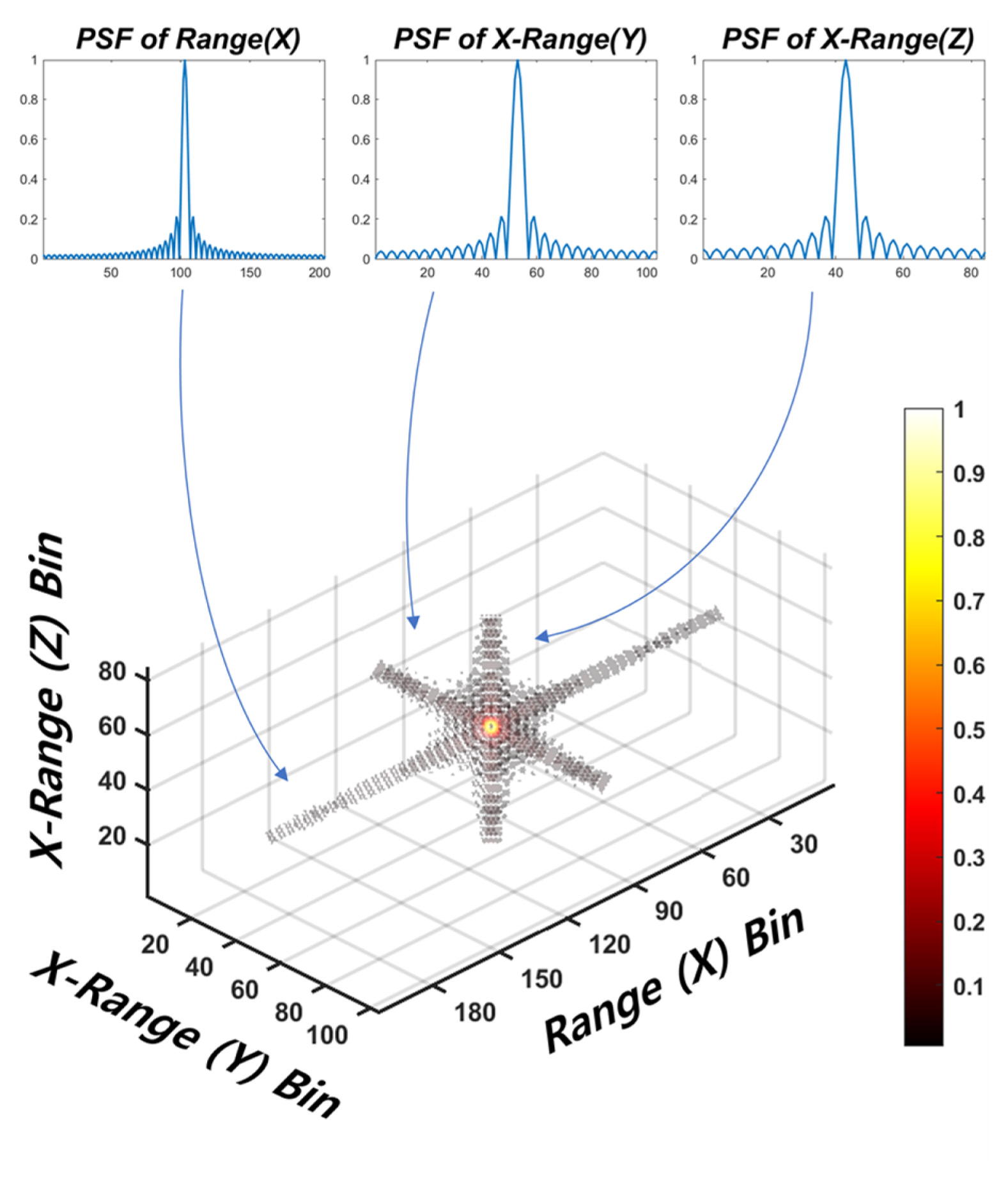
Configuration of a 3D volumetric scattering point.
In Eq. (8), the resolution of a 3D ISAR image is equal to the width of the main lobe of the sinc function, and Δx, Δy, Δz are defined as c⁄(2BW), c⁄(2fcΩ), c⁄(2fcΨ), respectively. The size of the volumetric scattering point becomes the resolution of the 3D ISAR image [1].
Fig. 2 shows a single volumetric scattering point located in a spatial domain consisting of one range and two cross-ranges. There is a sinc function in each axis direction. The properties of the scattering point depend on the radar parameters, and since sidelobes can be considered noise, various methods of removing them, such as bandpass filtering, have been investigated [1].
However, in the case of 3D ISAR images composed of these volume scattering points, image interpretation is more difficult than that entailed in HRRP or 2D ISAR imaging because the effects of clutter and backgrounds obscure the main scattering points. Therefore, it is essential to use the CLEAN method to reduce the effect of clutter. This application, in turn, improves the SNR and enables the mapping of only the primary scattering points to the spatial domain and their expression as volumetric scattering points [9, 10, 12, 13].
III. SIMULATION AND ANALYSIS OF RESULTS
Scattered wave signals for 3D ISAR formation were collected via simulation. The method of moments and the multilevel fast multipole method are widely used for scattering analysis [14]. However, these full-wave numerical analysis methods are deficient in that the calculation time increases rapidly as the number of meshes rises during high-frequency analysis or in cases wherein the target is relatively large.
These problems drove us to use ray launching geometrical optics (RL-GO), an approximation method similar to the shooting and bouncing rays method, which is specialized for high-frequency and large-target analysis [14, 15]. To this end, the radar parameters in Table 1 were used. A C-band (4–8 GHz) three times wider than the S-band (2–4 GHz) was used to analyze electrically large targets. Correspondingly, a 1/3 scaled model was used in the analysis [16].

ISAR parameters for simulation
Fig. 3 illustrates a simple-shaped perfect electric conductor CAD model of the Korma class used as a scatterer [17]. A scattered wave signal was collected using linear frequency modulation signal trains with a frequency of 5.75–6.75 GHz at an azimuth angle of −2.35° to 2.35° and an elevation angle of 72.8°–77.2°, as well as under the assumption of rotational motion by the target at sea. The 3D ISAR image with a resolution of Δx is 0.3 m, Δy is 0.3 m, and Δz is 0.32 m in the 3D ISAR dimensions of 15 m × 7.6 m × 6.5 m.
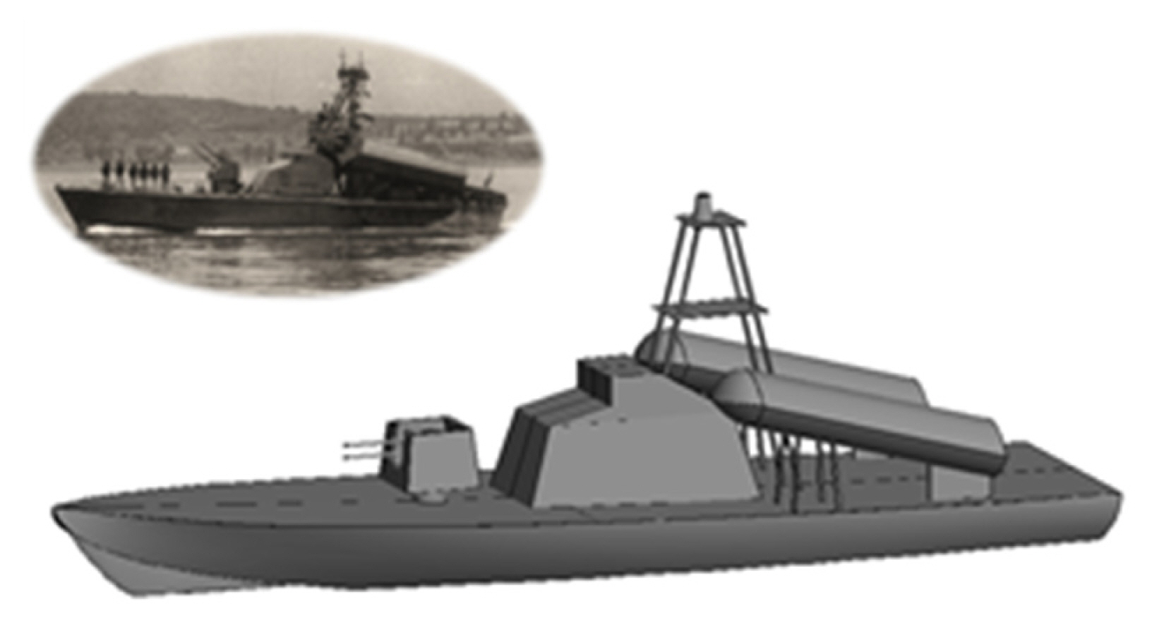
Fig. 4(a) shows the magnitudes of the HH-, HV-, VH-, and VV-polarized scattered electric fields. The figure indicates that the normalized magnitudes of the backscattered data differ depending on polarization characteristics. Fig. 4(b) shows an HRRP mapped with scattering points in the spatial domain. Similarly, it has different values depending on polarization characteristics, and the location of the scattering points is also different.
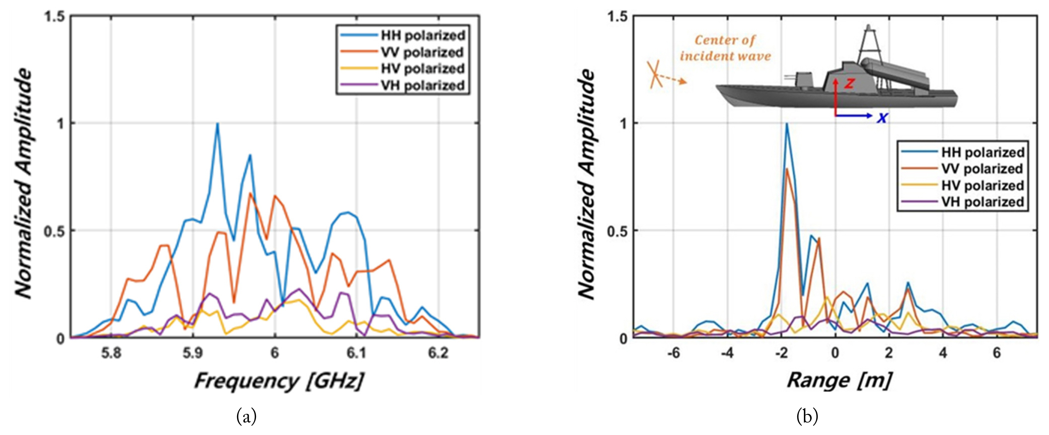
(a) Polarimetrically scattered electric field versus frequency and (b) 1D HRRP of the target (at azimuth angle: φc =0°; elevation angle: θc =75°).
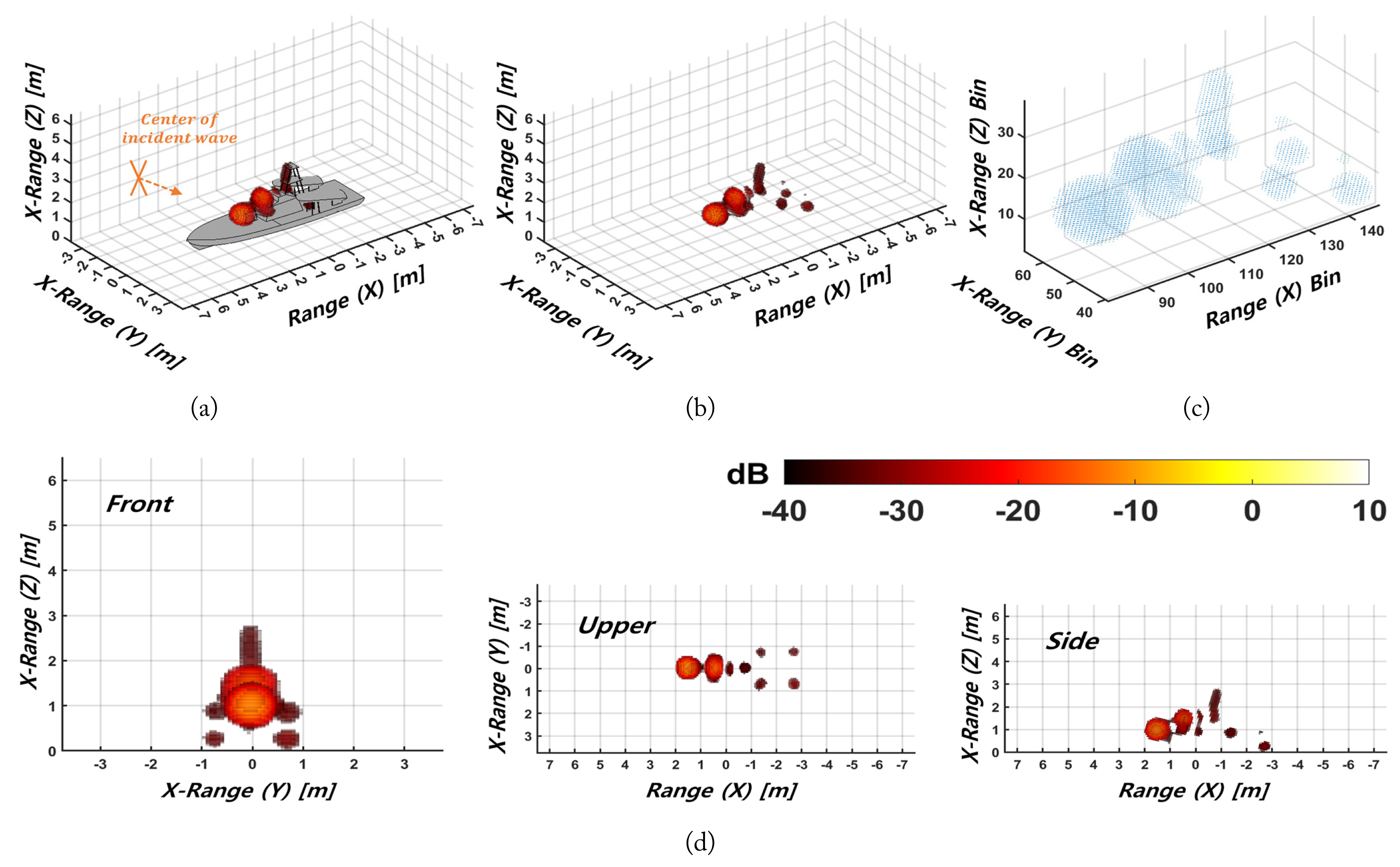
Fig. 5 depicts a 3D ISAR image formed using the scattered wave signals of HL polarization with a left-circular base transformed using HH- and HV-polarized scattered field data. Two polarized waves were compressed using Eq. (5), and the CLEAN method presented in Eq. (6) was used to reconstruct the image with a scattering point having a value over −40 dB. Only the main scattering points of the target are displayed, yielding an ISAR image that clearly shows morphological features. When evaluated against the CAD model, the scattering points are well formed, confirming that such points are concentrated on the deck, antenna, and missile launcher of the ship.

HL-polarized 3D ISAR images (a) with CAD model, (b) without CAD model, (c) scattering points cloud, and (d) 2D projections.
As shown in Fig. 5(d), the 3D ISAR image reconstructed with volumetric scattering points can form a 2D ISAR image projected onto the corresponding plane when observed in a direction perpendicular to each coordinate plane. In addition, a 2D ISAR image projected from a desired observation position can be acquired. It is easier to express the structural characteristics and scattering intensity of the target when a 3D ISAR is generated with volumetric scattering points than when it is formed with the scattering points cloud in Fig. 5(c).
Fig. 6 presents a 3D ISAR image created using the scattered wave signals of VL polarization converted using VH- and VV-polarized backscattered data. As reflected in Fig. 5(a) and 5(b), scattering points are formed mainly on the deck, antenna, and missile stand, but they also exhibit characteristics different from those of the scattered waves of HL-polarized data.
VL-polarized 3D ISAR images (a) with CAD model, (b) without CAD model, (c) scattering points cloud, and (d) 2D projections.
Fig. 7 compares the results before and after CLEAN application to the 3D ISAR image of the HL polarization in Fig. 5. Fig. 7(a) is the original 3D ISAR image, which is the result of directly applying IFT and includes noise in addition to the main scattering point of the target. Fig. 7(b), a 3D ISAR image constructed with the main volume scattering points using the CLEAN method, exhibits the main scattering points of the target. Applying the CLEAN method eases the capture of morphological characteristics by forming an image devoid of clutter around the target.
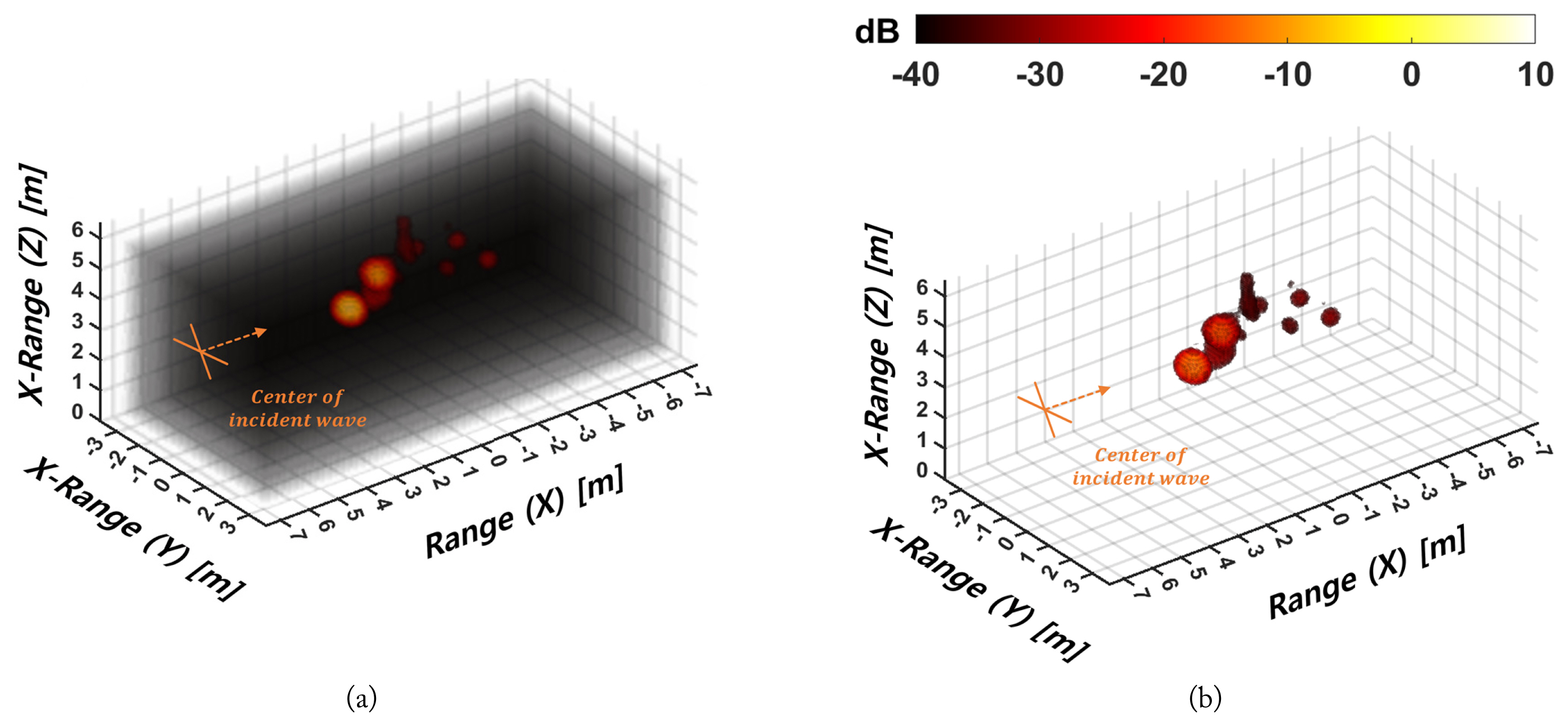
HL-polarized 3D ISAR images: (a) original 3D ISAR image of the target and (b) 3D ISAR image reconstructed with main scattering points using the CLEAN method.
IV. CONCLUSION
This study introduced a 3D ISAR image formation method that represents the intuitive shape and structural information of a target using monostatic radar. Scattered wave data collected on the basis of the rotational movement of a target can be mapped to the range and cross-range domains composed of a 3D Cartesian coordinate system through IFT. Each scattering point can then be defined as a PSF composed of a sinc function. In addition, the 3D ISAR image formed via volumetric scattering points can show more intuitive information on a target shape.
In radar equations, scattered electric field information has different characteristics depending on polarization. To use these equations, polarimetric ISAR data were employed. A 3D ISAR image was generated by compressing four linear polarization-based scattered waves expressed as a scattering matrix into two circular polarization-based scattered wave data.
The introduced algorithm produced results using backscattered data collected via simulation. Considering the size of the target, RL-GO, a numerical analysis method suitable for the target, was used. Scattered wave signals were collected using a full-wave electromagnetic simulator. Using the proposed algorithm enabled us to generate a 3D ISAR image that clearly shows the shape and structural characteristics of the CAD model.
In the formation of 3D ISAR images using bistatic ISAR or In-ISAR systems, researchers can model volumetric scattering points and map them onto a 3D coordinate axis [2, 3].
ACKNOWLEDGMENTS
This work was supported by the Aerospace Low Observable Technology Laboratory Program of the Defense Acquisition Program Administration and the Agency for Defense Develop-ment of the Republic of Korea.
References
Biography

Hyung-Jun Lee, https://orcid.org/0009-0008-1135-4150 received his B.S. degree in electrical and electronics engineering from the Republic of Korea Naval Academy, Jinhae, South Korea in 2017. He acquired his M.S. degree from Yonsei University, Seoul, South Korea in 2023. He is currently an officer in the Republic of Korea Navy. His research interests include RCS analysis and SAR/ISAR-ATR.

Yeong-Hoon Noh, https://orcid.org/0000-0003-3479-2838 received his B.S. and Ph.D. degrees in electronics engineering from Yonsei University, Seoul, South Korea in 2017 and 2023, respectively. He is currently a post-doctoral researcher at the Duke University, Durham, USA. His current research interests include RCS, numerical electromagnetics, and the design and analysis of microwave structures. His recent research focuses on RCS measurement for structures of various shapes and radar image processing based on scattering center modeling.

Jong-Gwan Yook, https://orcid.org/0000-0001-6711-289X was born in Seoul, South Korea. He received his B.S. and M.S. degrees in electronics engineering from Yonsei University, Seoul, South Korea in 1987 and 1989, respectively. He obtained a Ph.D. degree from the University of Michigan, Ann Arbor, USA in 1996. He is currently a professor with the School of Electrical and Electronic Engineering at Yonsei University. His research team recently developed various biosensors, such as carbon nanotube RF biosensors for nanometer-size antigen–antibody detection and remote wireless vital signal monitoring sensors. His current research interests include theoretical/numerical electromagnetic modeling and the characterization of microwave/millimeter wave circuits and components, the design of radiofrequency integrated circuits and monolithic microwave integrated circuits, and the analysis and optimization of high-frequency, high-speed interconnects, including signal/power integrity, based on frequency and domain full-wave methods.