


I. Introduction
Recently, a bandwidth required for measurement of a signal has been greatly increased in wireless communications and signal integrity. For example, USB 3.1 requires the measurement bandwidth of approximately 25 GHz. Thus, an oscilloscope capable of measuring a wideband signal is getting much attention. The oscilloscope that can measure these high frequency signals is divided into ŌĆ£real-timeŌĆØ and ŌĆ£sampling.ŌĆØ The traceable calibration methods for the real-time oscilloscope can be found in [1ŌĆō5].
A sampling oscilloscope operates on the basis of the principle of ŌĆ£equivalent time sampling,ŌĆØ and can digitize a fast signal of up to 100 GHz with a sub-picosecond sampling rate. However, this apparatus inherently has the systematic error time base distortion (TBD) in the sampling time [6].
There are various methods to calibrate TBD in the sampling oscilloscope such as ŌĆ£zero crossing,ŌĆØ ŌĆ£sine-fit,ŌĆØ and ŌĆ£analytic signal.ŌĆØ Among these, the sine-fit method is widely used due to its simplicity and robustness [7]. In-phase and quadrature (IQ) signals are usually fed into additional samplers (usually referred as the reference channel) to estimate TBD [8ŌĆō10]. Recently, the sample-time error has been considered as ŌĆ£errors in variableŌĆØ problem and is estimated using a software package for orthogonal distance regression (ODR), ODRPACK [11]. Thus, this method can calibrate TBD as well as random errors and does not require additional compensation for the random jitter, such as in [12].
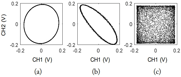
Some apparatus show high jitter between samplers [13]. Fig. 1 presents the IQ signal measured on various apparatus, and the measurement is mapped to the IQ domain. Therefore, the time information is eliminated and only the voltage value of each channel remains.
When the noise or the uncorrelated jitter between two channels becomes large, the line thickness of the circle becomes thicker. The method in [11] shows inaccurate results, as the non-common timing error increases, such as that shown in Fig. 1(b), since it assumes that the produced sample-time errors are almost the same on all reference channels.
In this paper, we propose an estimation method using multiple IQ signals of different frequencies to robustly calibrate TBD as well as random errors with relatively large independent timing errors. The multiple IQ signals have already been used in [8, 11], but they have only been adapted to reduce the ambiguity between TBD and the non-linearity of a sampler or to estimate the initial TBD. However, the proposed method can more accurately correct the nonlinearity of the sampler and the signal source by including the harmonic terms in the fitting model and it does not require the initial values in the fitting process. Unlike conventional methods, the simultaneously measured multiple IQ signals are used to minimize random errors by increasing the orthogonality of the basic functions in the fitting model.
This paper is organized in the following manner: Section II explains the error model for the systematic timing error in the sampling oscilloscope, the multiple IQ approach, and the uncertainty analysis. Section III provides optimum conditions, such as frequency selection on multiple IQ signals. Section IV presents the conclusion.
II. Estimation of Sample-Time Error
1. Error Model
The produced sample-time errors on each channel are composed of a systematic error TBD and random error Žäsampler (jitter of sampler), Žäsource (jitter of source), and Žätrigger (jitter of triggering circuitry), as shown in Fig. 2.
where j and i indicate the jth channel and ith sample index, respectively. If Žä(sampler)j,i and Žä(source)j,i are smaller than others, the timing errors ╬ötj,i can be approximated to TBDi + Žä(trigger)i. Thus, all channels have a common timing error that can be estimated using the IQ signal.
However, if the non-common error Žä(sampler)j,i and Žä(source)j,i are relatively larger than other errors, it cannot be estimated with the single IQ signal. In this case, multiple IQ signals are required to accurately estimate the common errors in the measurements. The regression is realized by the ODR, as explained in the next section. To suppress ambiguity of the measurement, the selected frequency is a slightly different frequency (this will be discussed in detail in Section III).
2. Estimation of Sample Time
The following fitting function is used in the estimation of the sample-time error:
where ╬┤i represents the summation of common timing errors TBDi and Žä(trigger)i. h means the number of harmonics generated by the source and non-linearity of the sampler, cj is the offset of the sampler, and ╔øj,i represents the residual errors with zero mean.
We estimate the timing error with the iterated ODR. The iterated ODR makes that
Žē ╬┤ Žā ╬┤ 2 Žē ╔ø Žā ╔ø 2 Žē ╬┤ Žā ╬┤ 2 / Žē ╔ø Žā ╔ø 2
Accordingly, G has the value of either +1 or ŌłÆ1, as
Žē ╬┤ Žā ╬┤ 2 / Žē ╔ø Žā ╔ø 2
3. Uncertainty Analysis
The uncertainty of the sample time errors in estimators can be considered as the non-linear ordinary least square problems in the following manner [15]:
Sparam in (5) is the covariance of the estimated parameters (ah,j, bh,j, cj, ╬┤i), and Žā2 is the residual variance of estimators; thus
Žā 2 = ( Žē ╬┤ Žā ╬┤ 2 + Žē ╔ø Žā ╔ø 2 ) / v
In this matrix, the covariance for the sample-time errors St is [
Žā ╬┤ 2
III. Optimum Conditions for Estimations
The timing error ╬┤ has a different effect on the measured value y depending on the signal g on ti, as shown below [9]:
where ╔ø is the noise, Žā is the variance of each variable, and gŌĆ▓(ti) is the derivative of input signal at time ti, respectively. Thus, the IQ signal with sine waveforms can produce orthogonal basis functions cos(Žē1t) and sin(Žē1t) in ODR fitting. The orthogonality of the basis function can be increased more by using the IQ signal with different frequencies. In this section, Monte-Carlo simulations are performed to obtain these optimal conditions. First, the condition for the frequency selection is addressed. Fig. 4 presents the residual estimated timing errors as the frequency of the additional reference channel changes. Here, 10 measurement sets are created, and each set comprises 20,000 data samples. The sample interval is 5 ps and the amplitude of reference signals are the same as those in the previous section. The 3 GHz and 11 GHz signals are used as the first reference signals in Fig. 4(a) and (b), respectively. In each Monte-Carlo simulation, the random errors are differently changed to achieve independence; ŽāTBD = 6.5 ps, ŽāŽäsampler = 2.5 ps, ŽāŽäsource = 0.2 ps, Žā╔ø = 0.004 V in Fig. 4(a) and ŽāTBD = 3.0 ps, ŽāŽäsampler = 1.0 ps, ŽāŽäsource = 0.2 ps, Žā╔ø = 0.008 V in Fig. 4(b). In the simulation, the result using the same frequency as the first reference signal also shows small residual errors that are different from the result in [8], since the proposed approach yields sample-time errors, including random errors, in addition to TBD. In both results, RMS residual errors are the smallest when the frequency of the second signal is approximately 1.1 times greater than the first reference signal.
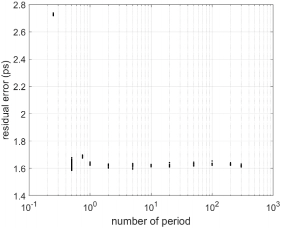
Next, the criterion for the number of periods is investigated. All conditions are the same as the simulation in Fig. 4(a), and the sample time is determined as Nperiod / L / freference. Nperiod is the number of periods and freference is the frequency of the first reference signal. In this simulation, the frequency of the first and second frequencies is set as 3 and 3.5 GHz, and the result is represented in Fig. 5. When the period is less than 0.5, the sine waveforms measured by reference channels are too short to be orthogonal to each other. However, the estimator can obtain a good estimation result when the reference signal is captured for at least one period on the oscilloscope display.
IV. Conclusion
In this paper, we propose an estimation method based on using the multiple IQ signals to evaluate the sample-time errors in the sampling oscilloscope. The estimator is implemented using the ODR and does not require any prior information. The numerical simulations reveal that the proposed method is more accurate than the method using only a single IQ signal when the independent jitter between the samplers is increased. It is also found that the frequency of the second reference and quadrature signals should be selected to be 1.1 times higher than the frequency of first ones. Moreover, the signals of approximately one period have to be captured on an oscilloscope display to adequately calibrate sample-time errors.