Estimation of Electromagnetic Properties for 2D Inhomogeneous Media Using Neural Networks
Article information
Abstract
Electromagnetic measurements are widely used to gain information about an object through interaction of electromagnetic fields with the physical properties of this object. The inversion problem is the process of estimating object parameters from electromagnetic records. This problem has a nonlinear nature and can be formulated as an optimization scheme. In this paper, we introduce an inversion methodology to estimate the electrical properties of a two-dimensional inhomogeneous layered scattering object. The proposed methodology deals with the inversion problem as a learning process through two multilayer perceptron artificial neural network designs. Several neural network design parameters were tuned to achieve the best inversion performance. Moreover, the proposed neural networks were tested against noise presence in terms of error criteria and proved to be effective in solving the inverse scattering problem.
I. Introduction
Over the past decades, electromagnetic methods have been widely used for medical, environmental, and engineering purposes [1]. Electromagnetic measurements collected at a receiver can be considered a set of electromagnetic field data scattered from an object and measured in time, frequency, or spatial domain [2]. Inversion is the process of estimating the physical parameters of an object from electromagnetic measurements [3]. Forward calculation, by contrast, denotes the simulation of electromagnetic measurements on a given object model, which is theoretically possible, provided that the relevant physical relations are known [4]. The relationship between the inverse and the forward problem is that the latter can be used to probe the former by testing suggested model parameters and assessing the sensitivity of the predictions of small changes in the parameters of this model [5]. The efficiency of the forward model will, therefore, strongly influence the efficiency of the inversion process, and can be used iteratively as part of the inversion process [6].
Thus, in this paper, we present a forward formulation for the calculation of the scattered electromagnetic field from an inhomogeneous layered-shaped scatterer. Considering the inversion methodology, an approach to representing the inversion scheme is adopted through a learning process in which the given input is a set of scattered field measurements, and the output is the model parameters. It is then necessary to find the configuration that can best map the input data to the output data [7]. This can be done using supervised learning techniques [8]. In this paper, we also present an inversion strategy to solve a two-dimensional electromagnetic inversion problem. A multilayer perceptron (MLP) artificial neural network is used as a learning process to solve the inversion problem. Several design factors were investigated to identify an optimal neural network design from an error analysis prospective to ensure the best performance. Furthermore, the performance of the selected neural network configuration was tested in the presence of noise, and the results are presented.
II. Forward Problem Formulation
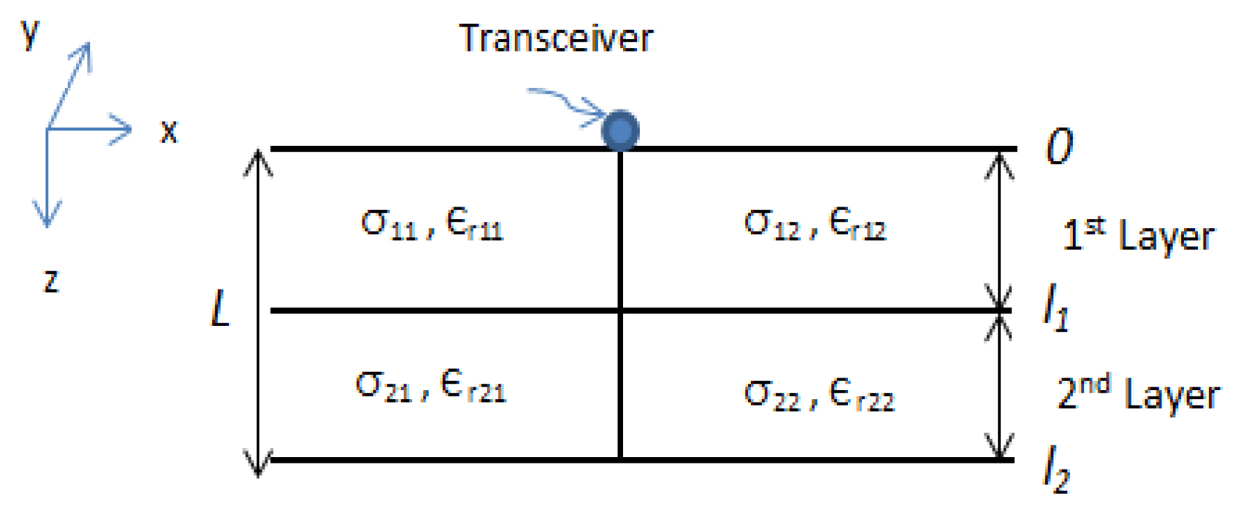
The solution to the forward scattering problem produces a scattered electric field measured at the point of interest on the interface [9]. In this paper, we consider an infinite unphased electric line source in the y direction acting as a transmitter leading to a transverse electric field in the y direction. We aim to compute the field scattered from the inhomogeneity back to the background medium. We limit our analysis to a two-dimensional (2D) inhomogeneous layered medium, that is, dielectric permittivity ɛ, and electric conductivity σ are inhomogeneous in z and x only. Further assumptions are that μ is everywhere equal to the permeability of free space μ0 (Fig. 1).
Therefore, for such a 2D problem and no magnetic currents, the non-vanishing field components are the electric field in the y-direction and the magnetic fields in the x and z directions [10]. If the scatterer presence can be thought of as an electric polarization current, J(x,z), The electric field inside the scatterer is given by [11]:
where Eym(x,z) is the total field inside the medium,
with lateral variations along the layered structure and the line source located at xs=zs=0, with
where
Therefore, Maxwell’s equations inside the scatterer are represented in the form of a volume integral equation on the electric polarization current [13]. We then solve the following integral equation:
using the eigensolution after normalizing wrt −iwμ0, we obtain:
where λn stands for eigenvalue and ψn stands for eigenfunction [14]. Now, we can make use of the eigenfunctions in the integral equation on Jy (kx, z) [15] represented by current expansion coefficients, an,m. Taking the inverse Fourier transform of both sides:
From the relation:
Multiplying by
where
We can then rewrite Eq. (12) to be:
Reforming Eq. (14) by approximating
where kxs = δ kxs and kxs′ = δ kxs′ and s = s″ − (S ″+1)/2 and s′ = s″ − (S′ + 1)/2, where s″ = 1, 2, …, S′ is an indexing parameter. This forms the linear system:
where a(kx) is a vector of length NS and c(kx) is a vector of length MS′. D(kx) is a square matrix with NS×MS′ dimensions, and c(kx) is an MS′ vector and can be constructed as:
I stands for the unit matrix of size MS′, and M is the total number of eigenfunctions to be included in the representation. a(kx) represents current expansion coefficients as:
Once we compute the coefficients {an(kx)}, the scattered electric field’s distribution is obtained at the receiver located at z = x = 0,
III. Inversion Approach
1. Data Preparation
An artificial neural network can be thought of as an input space mapping into a certain output space [17]. To simulate the required mapping, the network must be subjected to a learning process involving iterative changes to the internal parameters by presenting numerous input patterns with their consequent output patterns [18]. The training phase is achieved if the minimum error between the simulated output and the required output pattern is reached for all the training set’s examples. The network will afterwards simulate the required mapping on the training examples domain [19]. Neural networks have numerous uses, including time series prediction, function approximation, system control, and classification [20]. Artificial neural networks have also been widely used for solving inversion problems [21–24].
In this paper, an application of neural networks as an inversion scheme is presented, in which we design the network to receive input patterns in the form of scattered electromagnetic fields and produce the corresponding permittivities and conductivities as the material properties of a 2D inhomogeneous layered medium. The details of the proposed methodology are illustrated in Fig. 2.
The scattered fields were gathered for nine spatial harmonics. In the frequency domain, fields are represented by complex numbers that cannot be recognized as inputs to a single neural network. Thus, the real and imaginary components are separated to form an 18-input vector space dimension. We limit our case study to a two-layer model with a fixed layer depth resulting in eight output vector space dimensions. The eight outputs result from two neural networks that share the same 18 input vectors. The first network produces the estimated four permittivities values, and the second network produces the estimated four conductivities values (see Fig. 3). To ensure fairness, an output data set was prepared using a box-car random number generator Rand (1,1), with values ranging from zero to one. The generator was used to generate 254 examples as an output data set in the form:
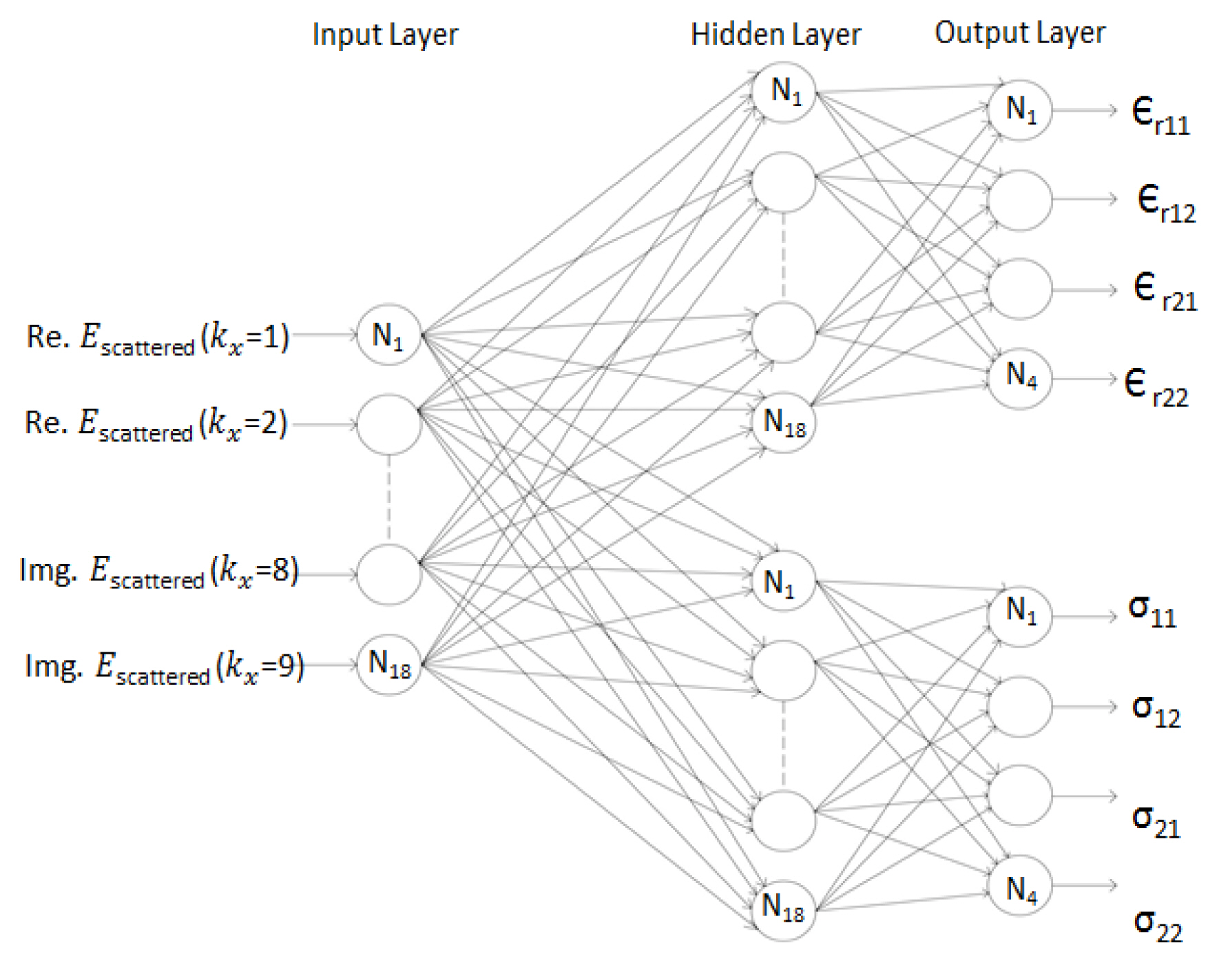
Proposed two neural network design models, each of which shares the same input layer with 18 nodes in each of its hidden layers. The first network output is the relative permittivities, and the second network output is the corresponding conductivities.
where ɛr,ij is the relative permittivity and σij is the conductivity with i,j=1,2, representing the vertical and horizontal inhomogeneity, respectively. Hence,
Table 1 shows the ranges of values for the relative permittivity and conductivity used in this paper.
2. Design Parameters
For the two neural network designs shown in Fig. 2, six design parameters were adjusted to achieve higher performance. The performance of the two neural networks was measured in terms of the upper and lower error bounds of each of the estimated parameters. These values are defined as:
where P represents one of the eight electromagnetic properties. n stands for the result estimated by the neural network, and m stands for the value on which the model was trained. eu corresponds to the max overestimate of the parameter, while el corresponds to the max underestimate of the parameter.
The first design parameter is the appropriate number of hidden layers and the number of hidden nodes in each layer. Several approaches have been used to relate hidden layer size to the number of nodes in the input and output layers. However, these approaches may not conform to all types of problems [25]. Thus, the most popular approach is trial and error. In this paper, both of the two proposed neural networks have one hidden layer with 18 neurons based on the sizes of the training set and input and output vector spaces, and they consider the tradeoff between the ability to interpolate and improve the fit (Fig. 3).
The second design parameter is the network training function. Five different training algorithms were used and compared in this paper: gradient descent with adaptive learning rate training “Tgda,” conjugate gradient backpropagation with Polak-Ribiére update training “Tcgp,” resilient backpropagation training “Trbp,” Levenberg-Marquardt backpropagation training “Tlmb,” and conjugate gradient with Fletcher-Reeves update training “Tcgf” [26].
Figs. 4 and 5 summarize the performance of the two neural networks in terms of the upper and lower error bounds of each of the eight estimated parameters against the suggested functions, while the other design parameters were kept fixed. It can be noticed that using the Levenberg-Marquardt backpropagation training function “Tlmb” yields significantly upper and lower error bounds for each of the estimated permittivities and conductivities values.
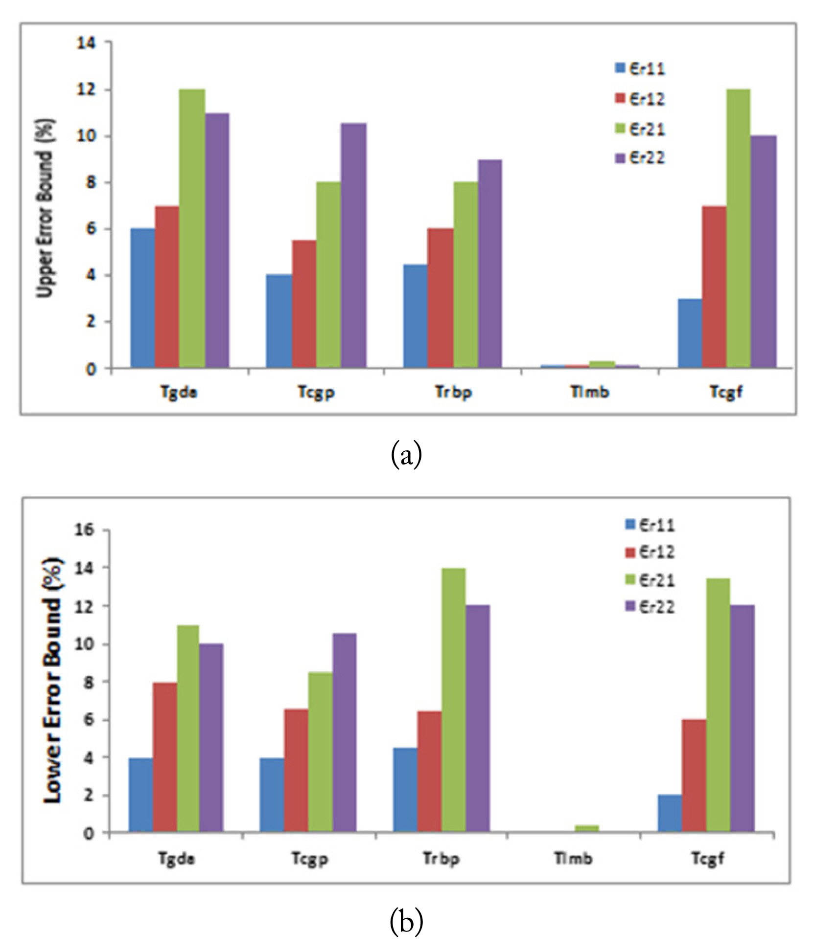
(a) Upper error bound and (b) lower error bound of each of the estimated relative permittivity against the suggested training functions, while other design parameters were kept fixed.
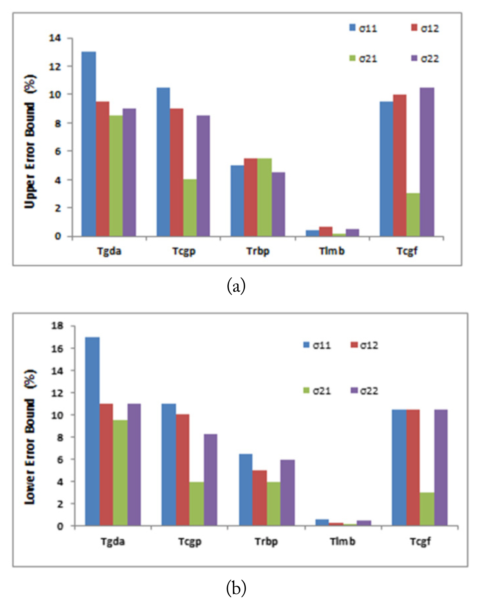
(a) Upper error bound and (b) lower error bound of each of the estimated conductivity against the suggested training functions, while other design parameters were kept fixed.
The third design parameter is the network learning algorithm. Five different learning functions have been used and compared in this paper: gradient descent with momentum weight and bias learning function “Lgdm,” Hebb weight learning function “Lhwl,” Kohonen weight learning function “Lkwl,” Perceptron weight and bias learning function “Lpwb,” and Instar weight learning function “Liwl” [27]. Figs. 6 and 7 summarize the performance of the two neural networks in terms of the upper and lower error bounds of each of the eight estimated parameters against the suggested algorithms, while the other design parameters were kept fixed. It can be noticed that both lower and upper error bounds reach a relatively small value when using the Hebb weight learning function “Lhwl” to estimate the permittivities values. However, the minimum lower and upper error bounds were achieved when using the perceptron weight and bias learning function “Lpwb” to estimate the conductivities values.
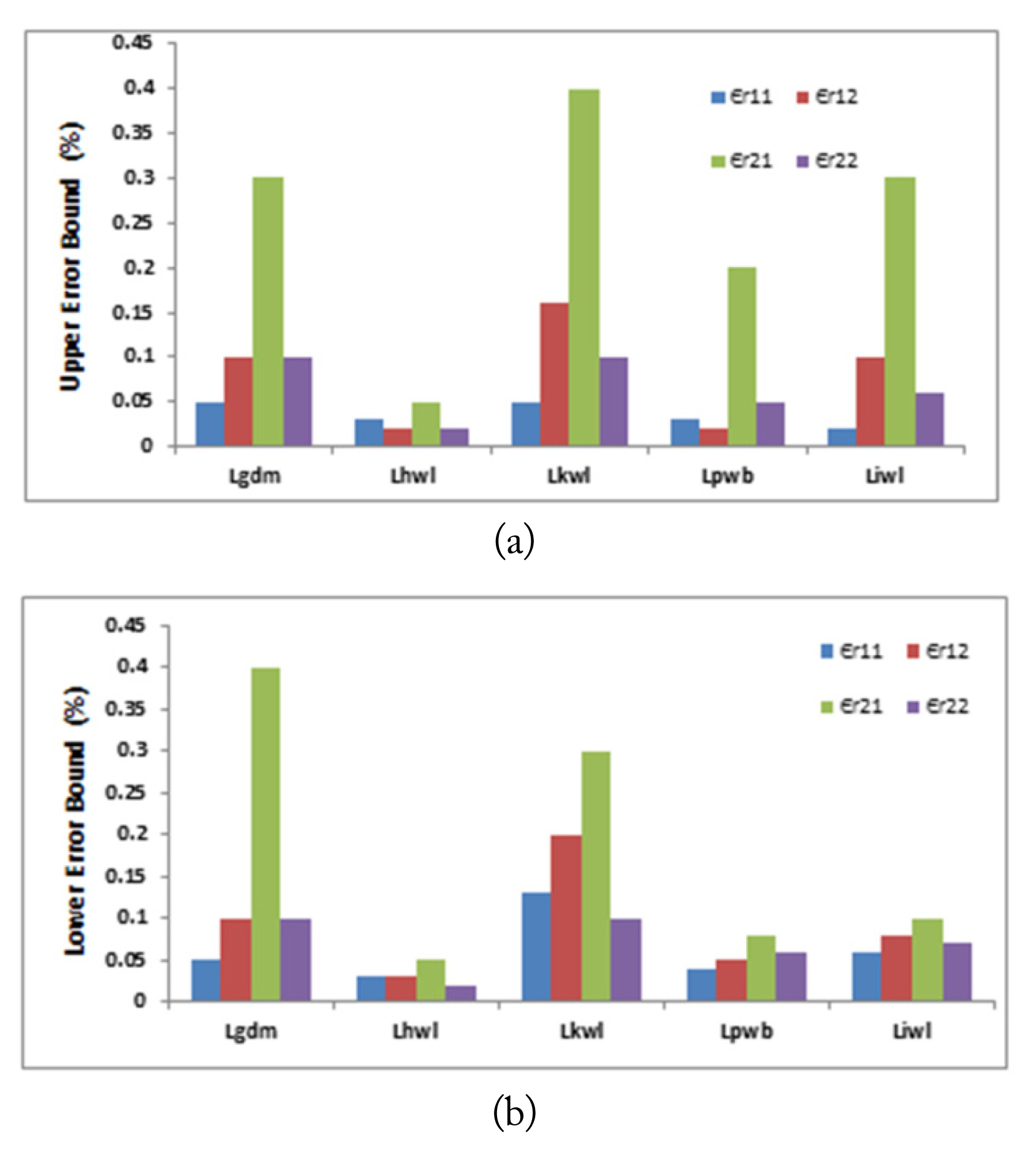
(a) Upper error bound and (b) lower error bound of each of the estimated relative permittivity against the suggested learning algorithms, while other design parameters were kept fixed.
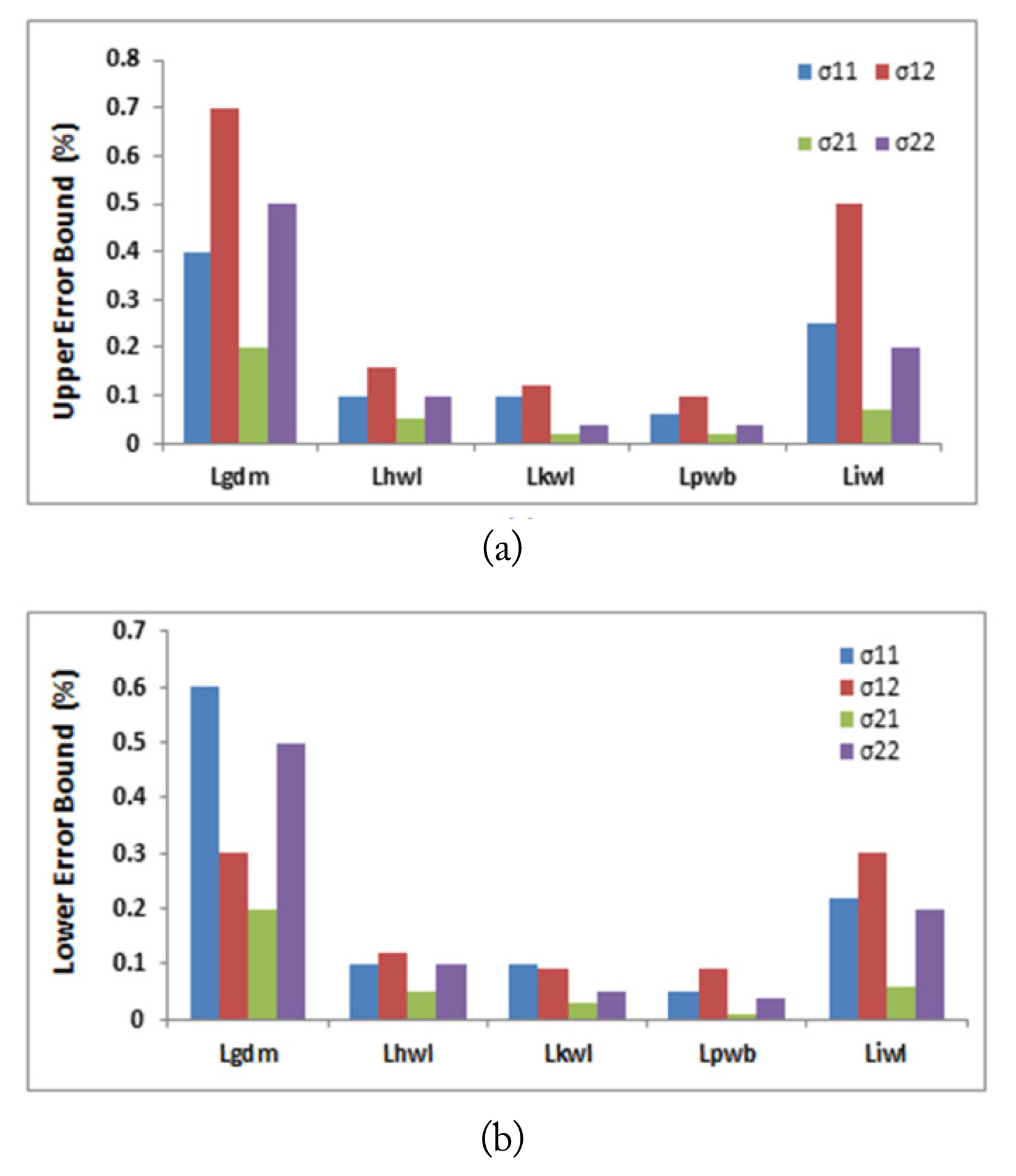
(a) Upper error bound and (b) lower error bound of each of the estimated conductivity against the suggested learning algorithms, while other design parameters were kept fixed.
The fourth design parameter is the size of the data subsets, which were randomly selected from the generated output data set—that is, the training Tt, validation Tv, and test Ts subsets. Although several approaches have been proposed regarding this issue, there are no mathematical rules for the required sizes of the various data subsets [28]. In this paper, the three subsets were randomly selected from the generated output data set.
The sizes of each of Tv and Ts subsets were set to be 25% and 25% of the size of Tt subset, respectively and were distinct from those examples selected for the training. Tables 2 and 3 represent the effect of Tt size as a percentage of the available output data set on the performance of the two neural networks, while the other design parameters were kept fixed. The fifth design parameter is the required number of iterations for proper generalization Itrn. For a given ANN architecture, this number can be determined by trial and error [29]. Figs. 8 and 9 represent the effect of Itrn on the two networks’ performance, while the other design parameters were kept fixed. As shown in the figures, there is a range of iterations in which the relative estimation error is minimized for each of the two networks. Fig. 8 shows that as the number of iterations increases, both the lower and upper error bounds decrease. However, the minimum lower and upper error bounds were achieved at the range between 1,700 and 2,000 iterations for the first neural network. By contrast, for the second neural network, the lower and upper error bounds reached their minimum at the range between 3,500 and 4,100 iterations, as shown in Fig. 9.

Effect of Tt size (%) of the available output data set on the permittivity network performance while the other design parameters are kept fixed

Effect of Tt size of the available output data set on the conductivity network performance while the other design parameters are kept fixed
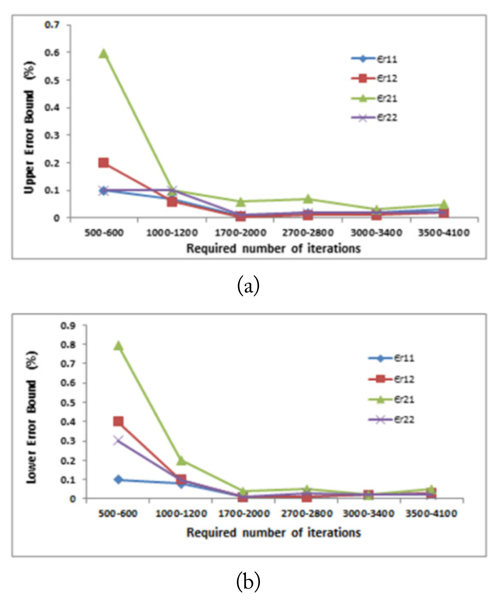
Effect of Itrn on the estimated relative permittivity while the other design parameters were kept fixed: (a) upper error bound and (b) lower error bound.

Effect of Itrn on the estimated conductivity while the other design parameters were kept fixed: (a) upper error bound and (b) lower error bound.
The sixth design parameter is the learning rate lr. Selecting a proper learning rate is a compromise between training acceleration and steady convergence [30]. Figs. 10 and 11 represent the learning rate effect on the two networks’ performance, while the other design parameters were kept fixed. As shown in Fig. 10, increasing the learning rate resulted in a decrease in both the upper and lower error bounds of the estimated permittivities. The minimum for both error bounds was achieved at a learning rate of 0.01. Beyond this value, both the upper and lower error bounds started to increase again.
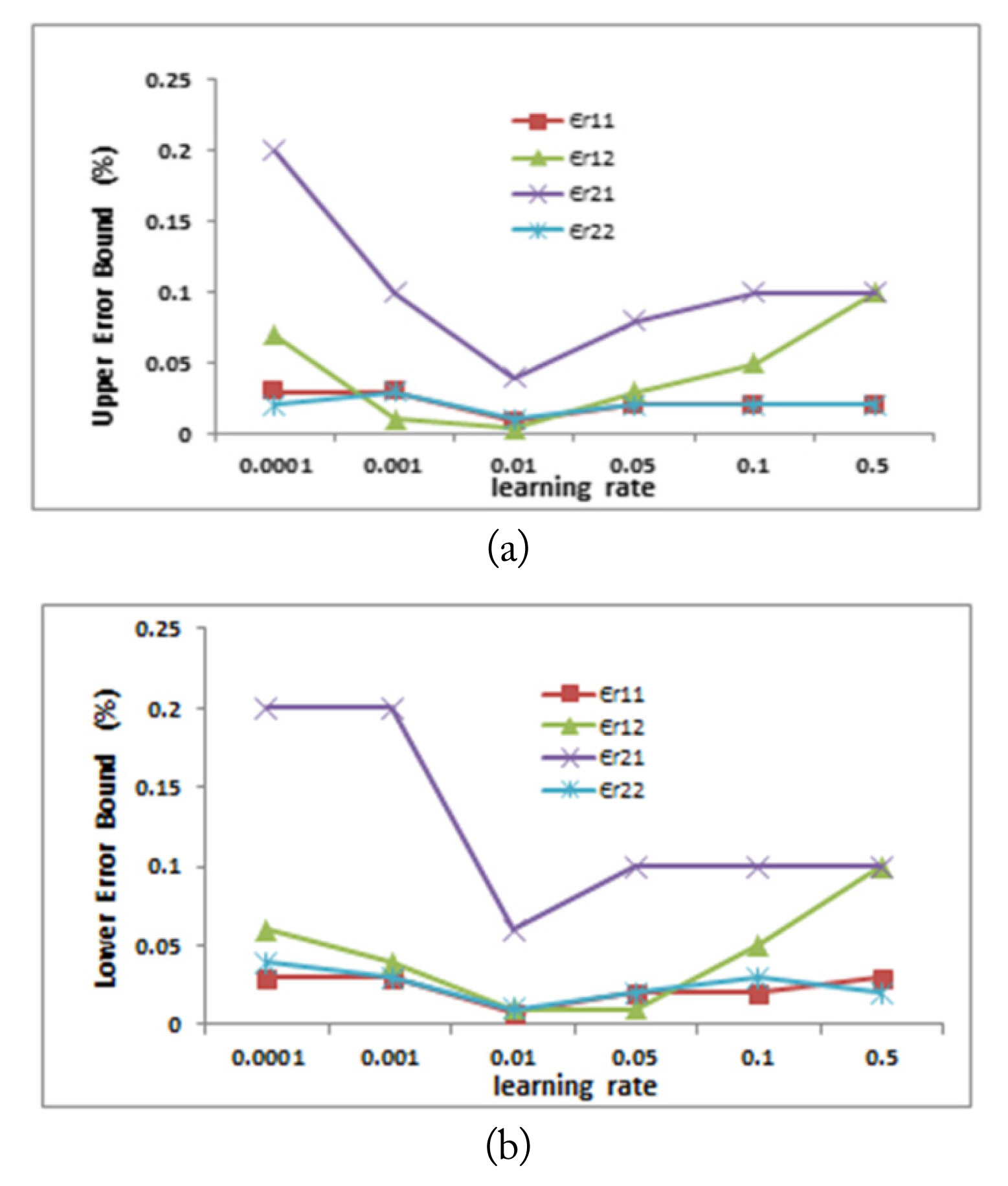
Effect of lr on the estimated relative permittivity while the other design parameters were kept fixed: (a) upper error bound and (b) lower error bound.
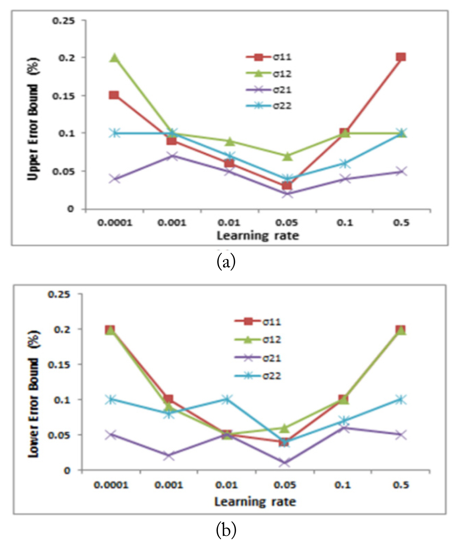
Effect of lr on the estimated conductivity while the other design parameters were kept fixed: (a) upper error bound and (b) lower error bound.
For the second neural network, it was observed that at a learning rate of 0.05, both the minimum upper error bound and minimum lower error bound were achieved for the estimated conductivities values, as shown in Fig. 11. Moreover, it was found that a further increase in the learning rate above 0.05 resulted in an increase in both error bounds.
IV. Results and Discussion
The selected design parameters, according to the studies presented in the previous section, for the two proposed neural networks are summarized in Table 4. It is considered that the percentage of training Tt, and test Ts data subsets that are randomly selected from the generated output data follow the box-car distribution of the original data set. Consequently, the network was not biased toward specific output data values compared to other output data values. Fig. 12 represents the performance of the two neural networks in terms of overall mean square error (MSE). We observed that using the selected design parameters, the performance goal of the two networks was relatively small.
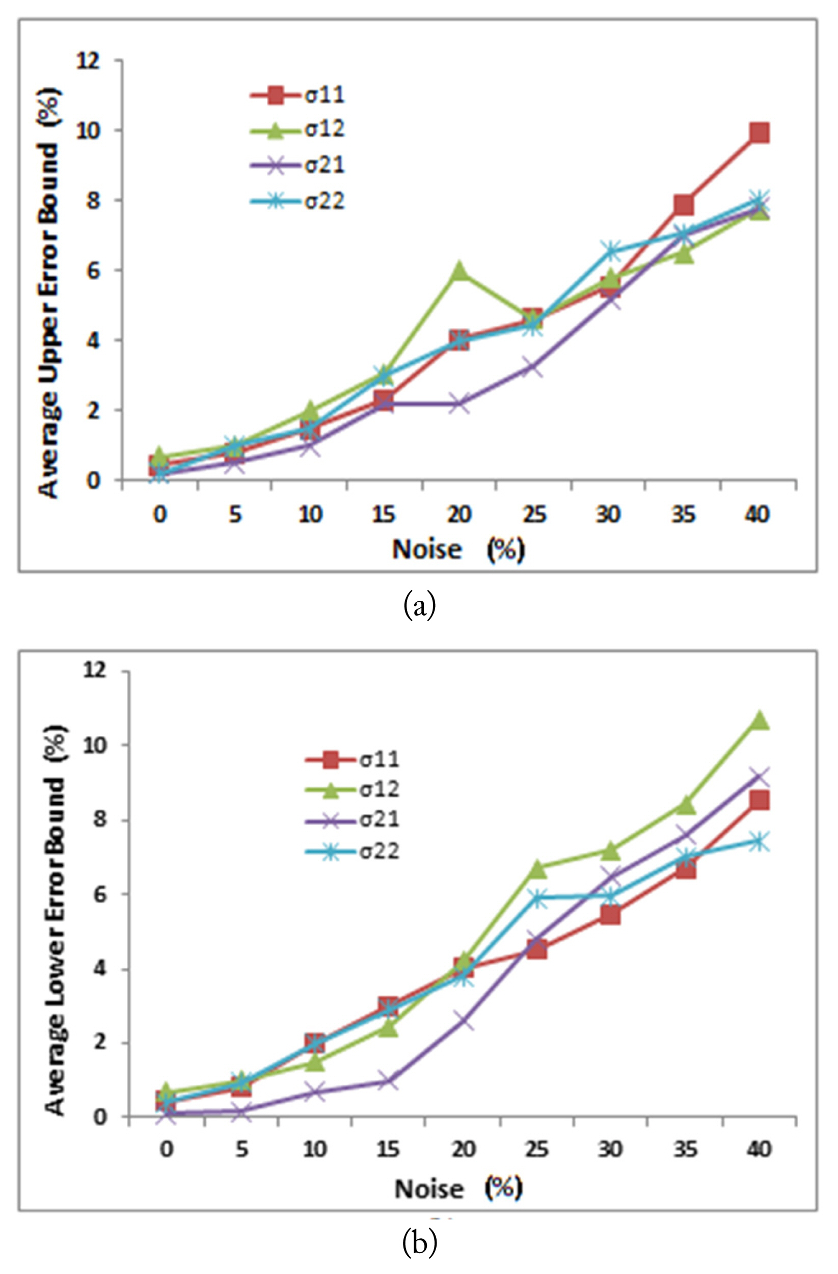
Starting from the selected design parameter indicators, the robustness of the two neural networks against noise was tested by adding different noise levels to the inputs of both networks using the box-car random number generator Rand (1,1) with various percentages to the training and test subsets. To evaluate the performance, we calculated the upper and lower error margins 100 times for each physical parameter of each layer against each noise level to form an average upper and lower error, as follows:
Figs. 13 and 14 show the two neural network performances in terms of average upper and lower error bounds for the test subset with the occurrence of noise. For the first neural network shown in Fig. 13, as the noise increased, the average upper error and average lower error bounds increased. Furthermore, as the noise value reached 40%, both average error bounds did not exceed 10%. The same trend was observed for the second neural network shown in Fig. 14, with a slight increase in both average error bounds values to reach 11% when the noise became 40%.
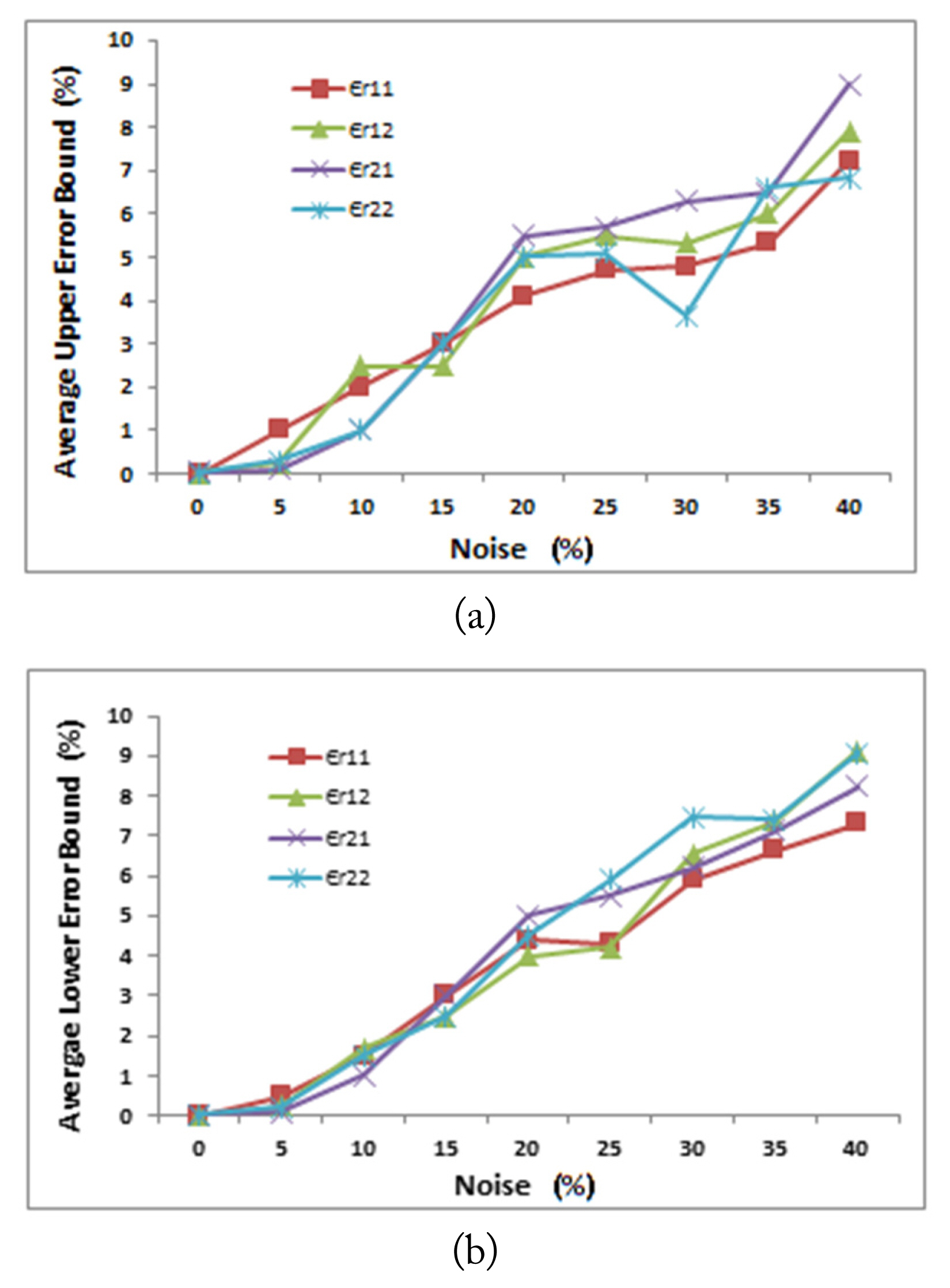
Effect of noise on the average upper error bound (a) and average lower error bound (b) of each of the estimated relative permittivities.
V. Conclusion
In this paper, a semi-analytical formulation for the forward calculation of the scattered electromagnetic field from a 2D inhomogeneous layered scattering object is presented. It involves a volume integral equation on an induced electric polarization current inside the scatterer and a complete orthonormal set of polarization currents to solve Maxwell’s equations. The proposed methodology in this paper offers a forward and inverse approach that can deal with structures in which permittivities and/or conductivities are function(s) of z and x directions per layer. The results of the proposed approach were used to generate the required data set for a MLP neural network. Two MLP neural networks were then designed to solve the inverse problem under consideration. Several design parameters were investigated and tested for optimal performance. The results showed that the trained networks were efficient in terms of error criteria and yielded accurate results, with an acceptable number of training examples. Further, the two proposed networks proved to be robust against several levels of noise, and their good interpolation ability was shown by the generalization results.
References
Biography

Mohamed Elkattan has been a lecturer at the Egyptian Nuclear Materials Authority since August 2013. He received his Ph.D. degree from Ain Shams University in Egypt in 2013. He received his M.Sc. degree in electronics and communications engineering from Cairo University, Egypt, in 2007. His research interests include antennas and wave propagation.

Aladin H. Kamel received a B.Sc. in electronics and communications engineering in 1975 (Distinction with Honors) and a B.Sc. in pure mathematics and theoretical physics in 1978 (Distinction with Honors), both from Ain Shams University, Cairo, Egypt. He conducted M.Sc. studies in electromagnetic boundary value problems at Ain Shams University and solid state physics at the American University in Cairo. He received a Ph.D. in Electrical Engineering from New York University, New York, USA in 1981. He won the best paper award from the Antennas and Propagation Society of the IEEE in 1981. He was an Assistant Professor of Electrical Engineering at New York University, a Manager of Research with the IBM Europe Science and Technology Division, and an executive manager with the Regional Information Technology and Software Engineering Center in Cairo, Egypt. His current research interests are in the areas of analytical and numerical techniques of radiation, scattering, and diffraction of waves, as well as inverse scattering problems.
